https://binds.cs.umass.edu/BrainPower/purplebrain.html
“We shall envision the mind (or brain) as composed of many partially
autonomous”agents”,
as a “Society” of smaller minds.
Each sub-society of mind must have its own internal epistemology and
phenomenology,
with most details private,
not only from the central processes,
but from one another.”
(Minsky, K-Lines; 1980)
Lesson in neuronal politics:
Strong local/individual policies have many strengths:
sustainable, realistic, flexible, robust, and fault-tolerant.
At the end of this section you should be able to:
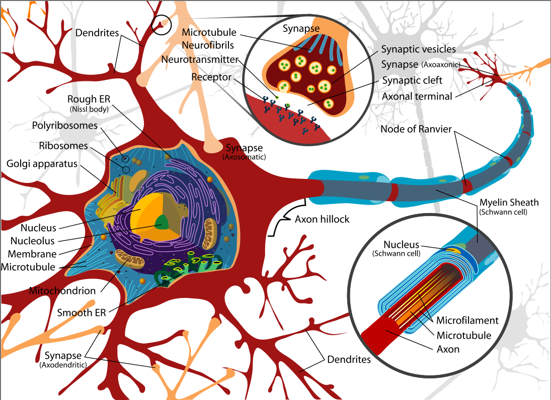
Real neurons
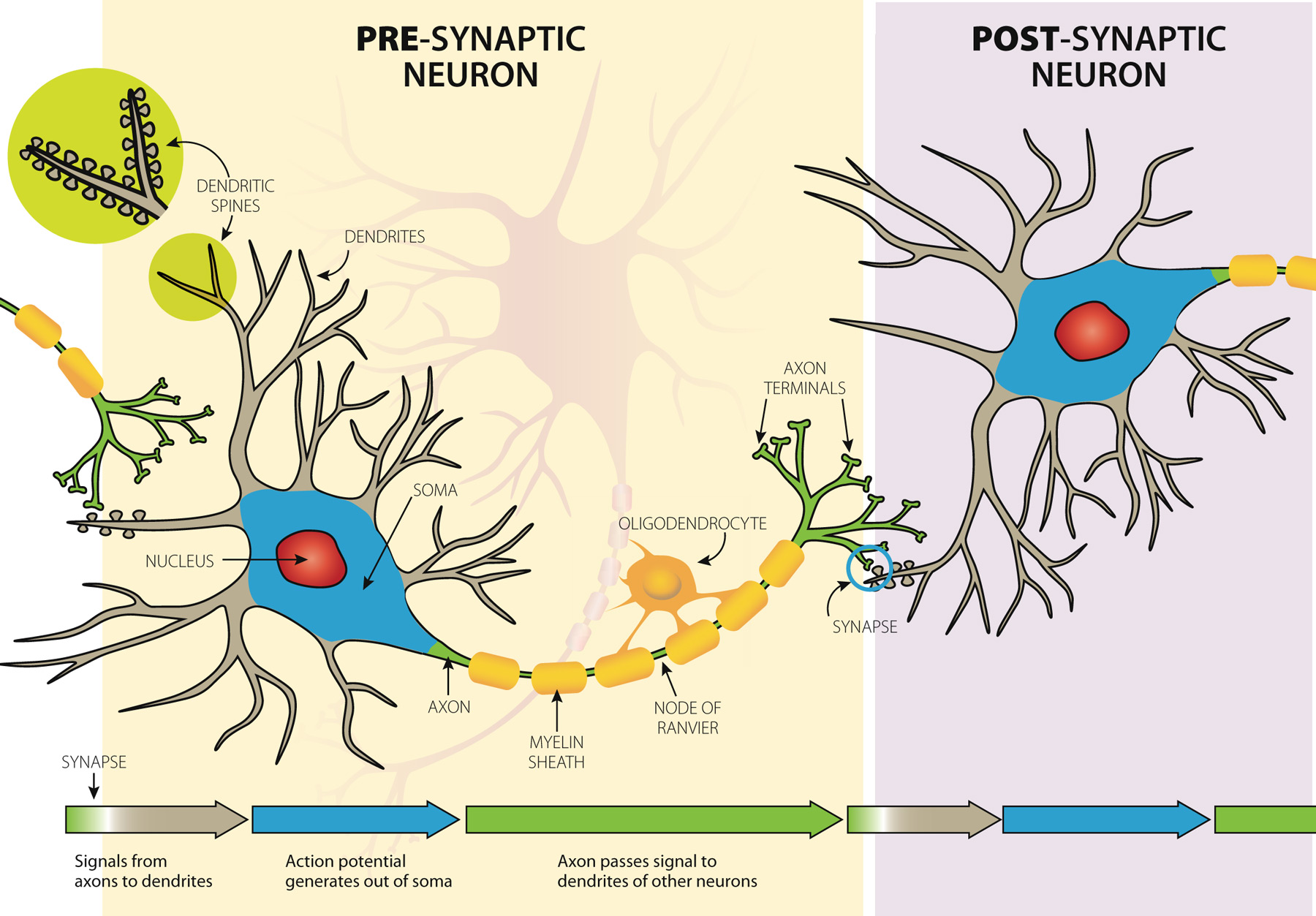
Pre- and Post- synaptic
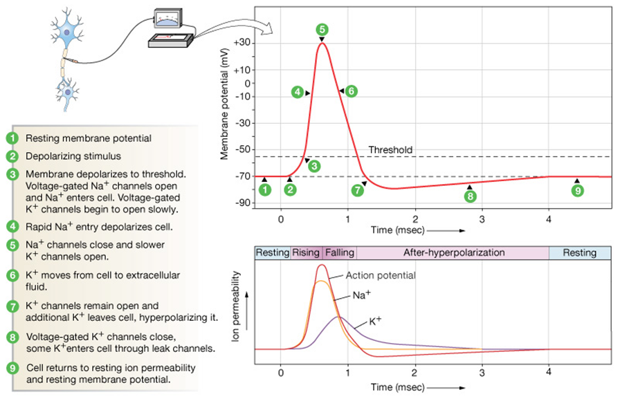
Action potentials
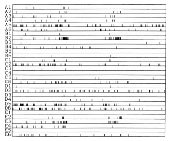
A 4 second recording of neural activity,
recording from 30 neurons (rows) of the visual cortex of a monkey.
Each vertical bar indicates a spike.
The human brain can recognize a face within 150ms,
which correlates to less than 3mm in this diagram;
dramatic changes in firing frequency occur in this time span,
neurons have to rely on information carried by solitary spikes.
How many neurons, or “hops” does it takes until recognition occurs?
Neurons spike to “think” (mostly)
Neurons are the primary basis of human/animal thinking, learning,
consciousness, etc.
Synapses: inter-neuron signaling / learning
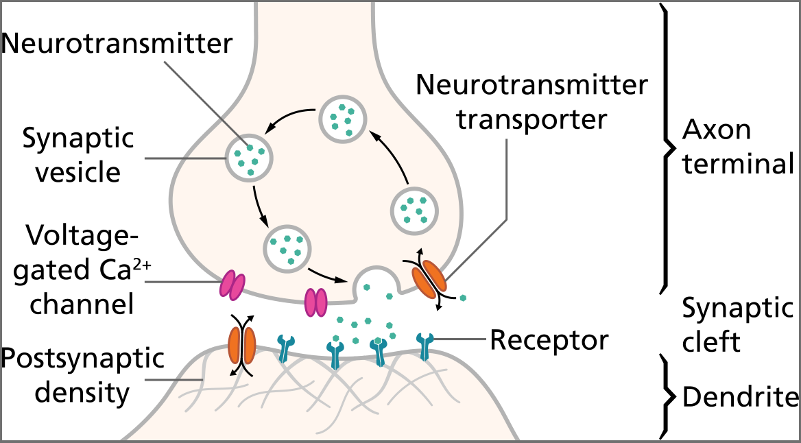
Rate-limited step is transmission between neurons.
Learning is mostly rooted in the synapses.
Neurons change their reactivity and “weights” to learn.
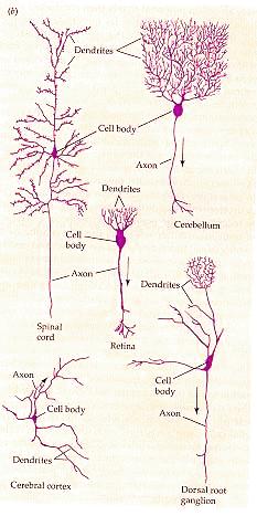
Diversity of neuron types
“What magical trick makes us intelligent?
The trick is that there is no trick.
The power of intelligence stems from our vast diversity (and
size),
not from any single, perfect principle.”
(Marvin Minsky, Society of Mind; 1987)
Diversity of neuron types cont…
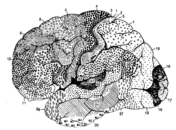
Network structure varies on a macro scale.
Level of abstraction
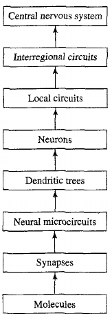
Which level of abstraction to model?
Discuss: Cortical columns as an expandable, general-purpose module.
Neurons are slow and fairly small:
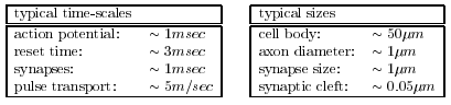
Compared to computers at least…
Brains vs. Computers
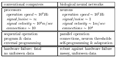
| × | process elements | element size | speed | computation | robust | learns | intelligent, conscious |
|---|---|---|---|---|---|---|---|
| Brain | 10^14 synapses | 10e-6m | 100Hz | parallel, distr | yes | yes | usually… |
| Computer | 10^8 transistors | 10e-6m | 10^9 Hz | serial, central | no | a little | Debateably yes |
Performance degrades gracefully under partial damage.
In contrast, most programs and engineered systems are brittle:
If you remove some arbitrary parts,
very likely the whole will cease to function.
Brain reorganizes itself from experience.
It performs massively parallel computations extremely efficiently.
For example, complex visual perception occurs within less than 30
ms,
that is, potentially 10 processing steps!
Brain is flexible, and can adjust to new environments.
Can tolerate (well) information that is fuzzy,
inconsistent, probabalistic, noisy, or inconsistent.
Brain is very energy efficient.
Traditional computing excels in many areas, but not in others.
A funny definition:
AI is the the development of algorithms or paradigms that require
machines to perform cognitive tasks at which humans are currently
better.
Symbolic rules don’t reflect processes actually used by humans.
Types of computation
Neural networks can be universal general purpose computers,
and in some app-specific hardware instances do better than Turing
machines.
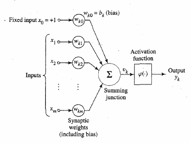
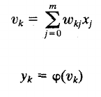
of neurons
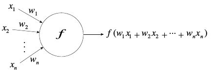
Neuron operations:
1. Sum (inputs x weights)
2. Apply activation function
3. Transmit signal
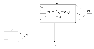
* Often a bias \(\theta\) can be
applied/learned
Many types:
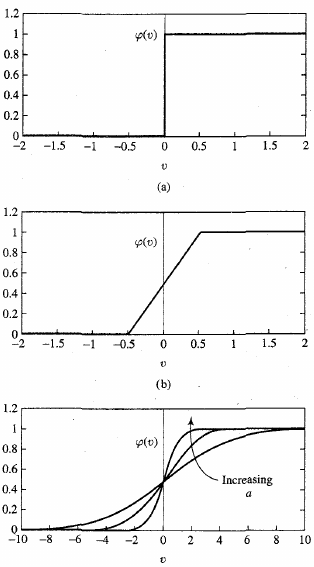
top above
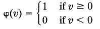
middle above
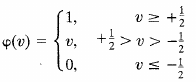
bottom above
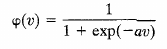
Note: \(exp(x)\) is \(e^x\)
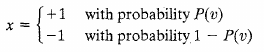
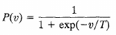
T is pseudo temperature used to control noise level (uncertainty)
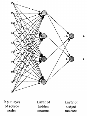
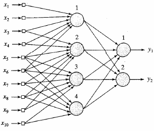
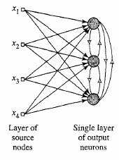
Signal flow diagram
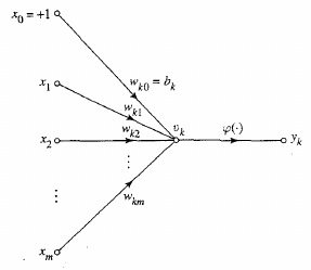
Graph structure
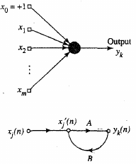
Single layer network
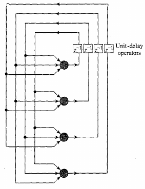
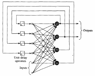
Recurrent network with no self feedback
Knowledge representation?
newsgroup example
Knowledge refers to stored information used to interpret,
predict, or respond to the outside world.
In a neural network:
* Similar inputs should elicit similar activations/representations in
the network
* The inverse: dissimilar items should be represented very
differently
* Important features should end up dominating the network
* Prior information can be built into the network, though it is not
required, e.g., receptive fields
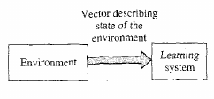
Learning is a process by which the free
parameters,
synaptic weights, of the network are adapted,
through a process of stimulation/activation,
by the environment in which the network is embedded.
The type of learning is determined by the ways the parameters are
changed:
Supervised (with sub-types),]
Unsupervised (with sub-types), and
Reinforcement learning.
A set of well-defined rules for updating weights is defined as a learning algorithm.
The mapping from environment to network to task is often coined the learning paradigm.
Unsupervised learning
E.g., clustering, auto-associative, Hebbian, etc
https://en.wikipedia.org/wiki/Hebbian_theory
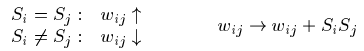
Neurons that “Fire together, wire together”.
Recall our basic neuron:
With pre-synaptic inputs (xn),
and post-synaptic output (y).
\(\Delta w_i = \eta x_i y\)
the change in the ith synaptic weight wi,
is equal to:
a learning rate \(\eta\),
times the ith input xi,
times the postsynaptic response y.
Weights updated after every training example.
Variants of this are very successful at clustering problems,
and can provably perform ICA, PCA, etc.
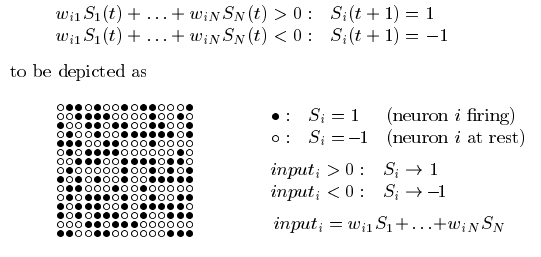
Hebbian-like rule:
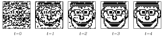
First the learning phase, when like activations become more
linked.
After learning, a partial activation will produce activity in neurons
more closely linked.
Thus, during this phase a partial noisy degraded image can produce
activations like that of the full image.
This is probably the best way to see parts of cortical
function!
Much of learning is driven by coincidence detection with massive
cross-referencing.
During recognition, behavior is thus like the associative example above,
in time and space.
See upcoming spiking networks lectures.
Structural: Which weights need changing due to good/bad outcome?
Temporal: Which preceding internal decisions resulted in the delayed reward?
One way of learning with a teacher (an involved, micromanaging
teacher).
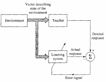
Supervised learning:
attempts to minimize the error between the actual outputs,
i.e., the activation at the output layer,
and the desired or “target” activation,
by changing the values of the weights.
Competitive learning
Winner-takes all based weight updates
(inhibition of lateral neighbors).
Similar to functions in retina
How much should we change each weight?
In proportion to its influence on the error.
The bigger the influence of weight wi,
the greater the reduction of error that can induced by changing it
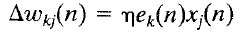
For a given learning instance, input n:
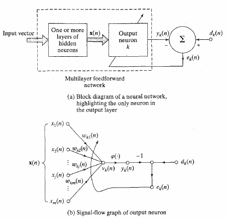
Error:
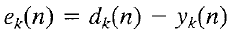
Minimize this error:
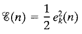
Update via:

After a hypothetical learning example,
below is some possible resulting weights and biases (theta).
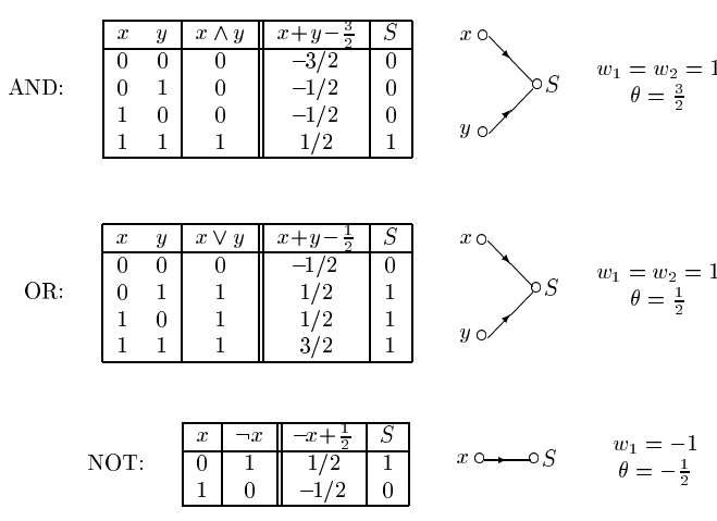
Easy for linear single layer network,
with 2 neurons and a bias,
with step activation.
XOR
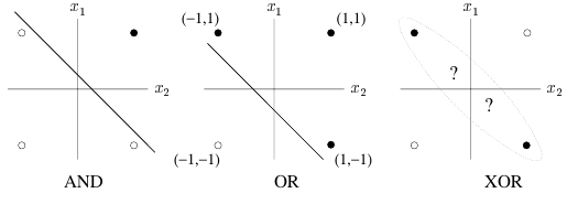
Problem:
Requires a hidden layer (for non-linearity)
Solution: N-layer network
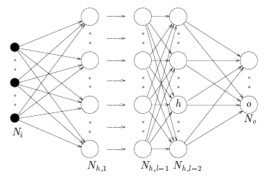
Solution: Can solve any non-linear function
XOR
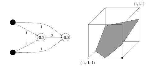
Separation into 3D via hidden layer allows solving XOR
Problem:
How to solve for errors in hidden layer??
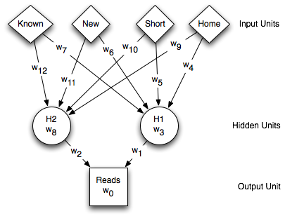
Neural network for traveling example
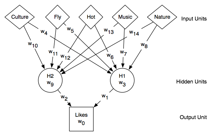
Neural network for traveling example
Given input example, \(e\), what is
output prediction?
Error gradients
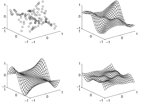
Top left: original samples;
Top right: network approximation;
Bottom left: true function which generated
samples;
Bottom right: raw error
Error gradients: simple
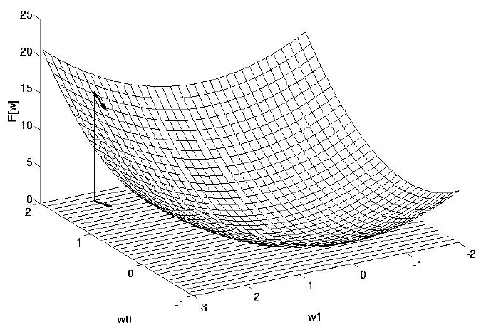
* Error (vertical) as function of 2 weights (\(x_1\) and \(x_2\))
Error
* How much should we change each weight?
* In proportion to its influence on the error.
* The bigger the influence of weight \(w_m\) , the greater the reduction of error
that can induced by changing it
* This influence wouldn’t be the same everywhere: changing any
particular weight will generally make all the others more or less
influential on the error, including the weight we have changed.
Solution: Error backpropagation
Each propagation involves the following:
Forward propagation of a training pattern’s input through the neural
network,
in order to generate the propagation’s output activations.
Backward propagation of output activations through the neural
network,
using the training pattern target,
in order to generate the deltas of all output and hidden neurons,
(delta is the difference between the input and output values)
For each weight-synapse do the following:
* Multiply its output delta, and input activation, to get the gradient
of the weight.
* Subtract a ratio (percentage) of the gradient from the weight.
Learning rate
The ratio (percentage) influences the speed and quality of
learning;
it is called the learning rate.
The greater the ratio, the faster the neuron trains;
the lower the ratio,
the more accurate the training is.
The sign of the gradient of a weight indicates where the error is
increasing,
this is why the weight must be updated in the opposite direction.
Finally:
Repeat step 1 and 2 until the performance of the network is
satisfactory.
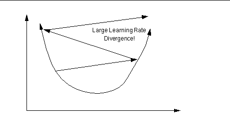
Learning rate is too large
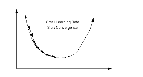
Learning rate is too small
Solution:
Error backpropagation overview and basic idea:
1 initialize network weights (often small random values)
2 do
3     for Ēach training example ex
4         prediction = neural-net-output(network, ex) // forward pass
5         actual = teacher-output(ex)
6         compute error $(prediction - actual)$ at the output units, as $\triangle$
7         Starting with output layer, repeat until layer I (input):
7             propagate $\triangle$ values back to previous layer
9             update network weights between the two layers
10 until all examples classified correctly or another stopping criterion satisfied
11 return the network
Backprop(from ArtInt)
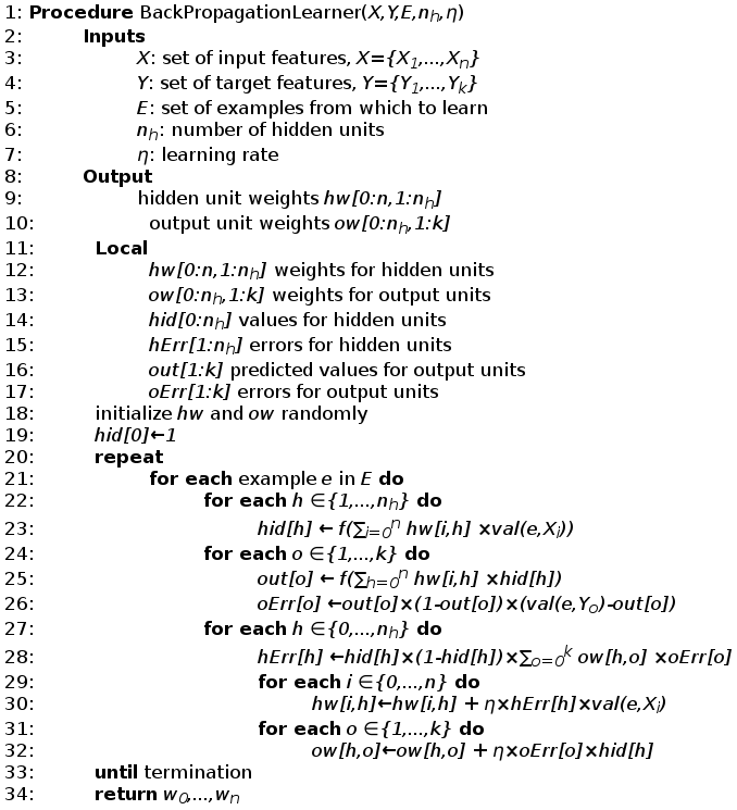
This approach assumes:
\(n\) input features,
\(k\) output features, and
\(nh\) hidden units.
Both \(hw\) and \(ow\) are two-dimensional arrays of weights.
Note that
\(0:nk\) means the index ranges from
\(0\) to \(nk\) (inclusive), and
\(1:nk\) means the index ranges from
\(1\) to \(nk\) (inclusive).
This algorithm assumes that \(val(e,X_0)=1\) for all \(e\)
Backprop (from AIMA)
Neural network for traveling example
One hidden layer containing two units,
trained on the travel data, can perfectly fit.
One run of back-propagation with the learning rate η=0.05, and taking
10,000 steps,
gave weights that accurately predicted the training data:
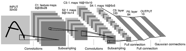
Comparison: digit recognition
| 3 NN | 300 Hidden NN | LeNet | Boosted LeNet | SVM | Virtual SVM | Shape match | |
|---|---|---|---|---|---|---|---|
| Error rate | 2.4 | 1.6 | 0.9 | 0.7 | 1.1 | 0.56 | 0.63 |
| Run time | 1000 | 10 | 30 | 50 | 2000 | 200 | • |
| Memory req | 12 | .49 | 0.012 | 0.21 | 11 | • | • |
| Training time | 0 | 7 | 14 | 30 | 10 | • | • |
| % rejected to reach 0.5% | 8.1 | 3.2 | 1.8 | 0.5 | 1.8 | • | • |
Prediction!
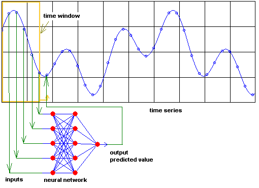
Neural networks can predict complex time-series, e.g., prices,
economies, etc
Prediction!
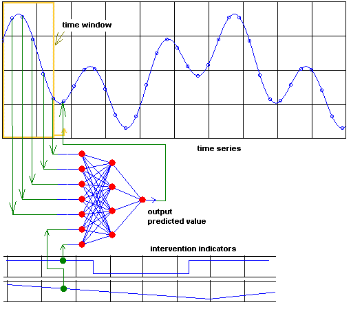
Input can be given by experts via intervention indicators
Prediction!
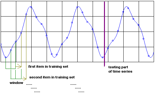
Training via a shifting window
Prediction!
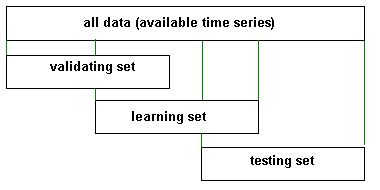
Like other methods, training, validation, and testing sets help
Another way of learning with a teacher (a negligent, rarely-there
teacher).
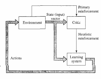
Temporal credit assignment problem.
More to come with spiking networks.
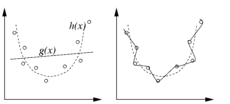
* Over-fitting impedes generalization
Regularization
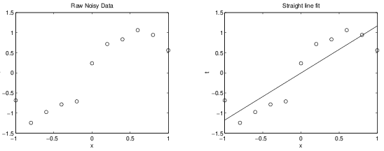
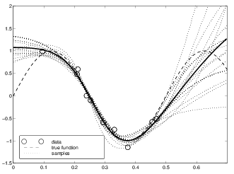
Straight line might be an under-fit to these data points.
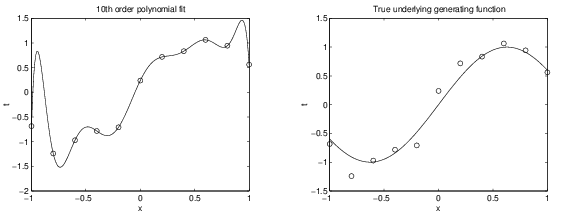
Left, 10th order might be an over-fit.
Right, the true function from which the data were sampled.
Regularization
\(\lambda\) defined as a constant to
penalize higher order during the error calculation (for neurons)
Regularization:
too little or too much
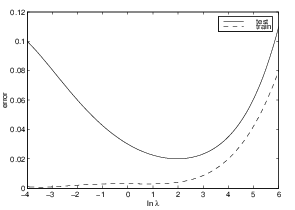
* dotted = train, solid = test
* y=error, x= \(\lambda\), such that
either too low or high order is worse, with a happy medium in the
middle.
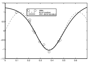
Regularization: Bayesian
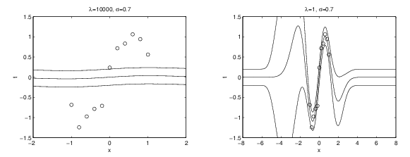
* Pre-specify your hypothesis about \(\lambda\)
* Left, \(\lambda\) 1000
* Right, \(\lambda\) 1
Regularization: Bayesian
* \(p(w|\lambda, H) \propto
exp[-\frac{\lambda}{2}w^2]\)
* \(p(\textbf{w}|D, \lambda, H) = \frac{
p(D|\textbf{w}, \gamma, H) p(\textbf{w}|\lambda, H)}{p(D|\lambda,
H)}\) such that \(D\) are
data
* \(p(\textbf{w}|D, \lambda, H) =
p(D|\textbf{w}) \propto \prod_u
exp[-\frac{1}{2}(y^u-f(x^u-\textbf{w}))^2]\)