Discrete Mathematics using a Comptuter (O’Donnell, Hall, Page) Chapter 2
Discrete Mathematics with Applications - Metric Edition (Epp) Chapter 1
https://runestone.academy/ns/books/published/DiscreteMathText/chapter1.html
https://runestone.academy/ns/books/published/DiscreteMathText/variables1-1.html
https://runestone.academy/ns/books/published/DiscreteMathText/lang_sets1-2.html
https://runestone.academy/ns/books/published/DiscreteMathText/lang_relations1-3.html
https://www.cs.carleton.edu/faculty/dln/book/ch02_basic-data-types_2021_October_05.pdf
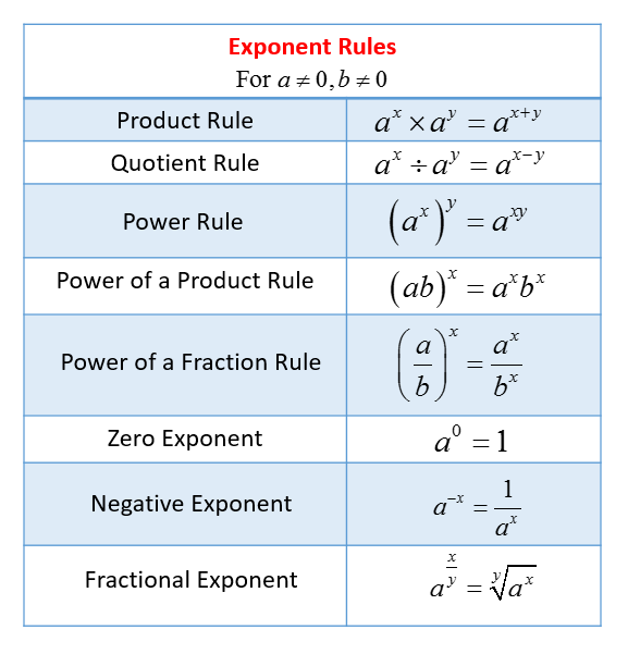
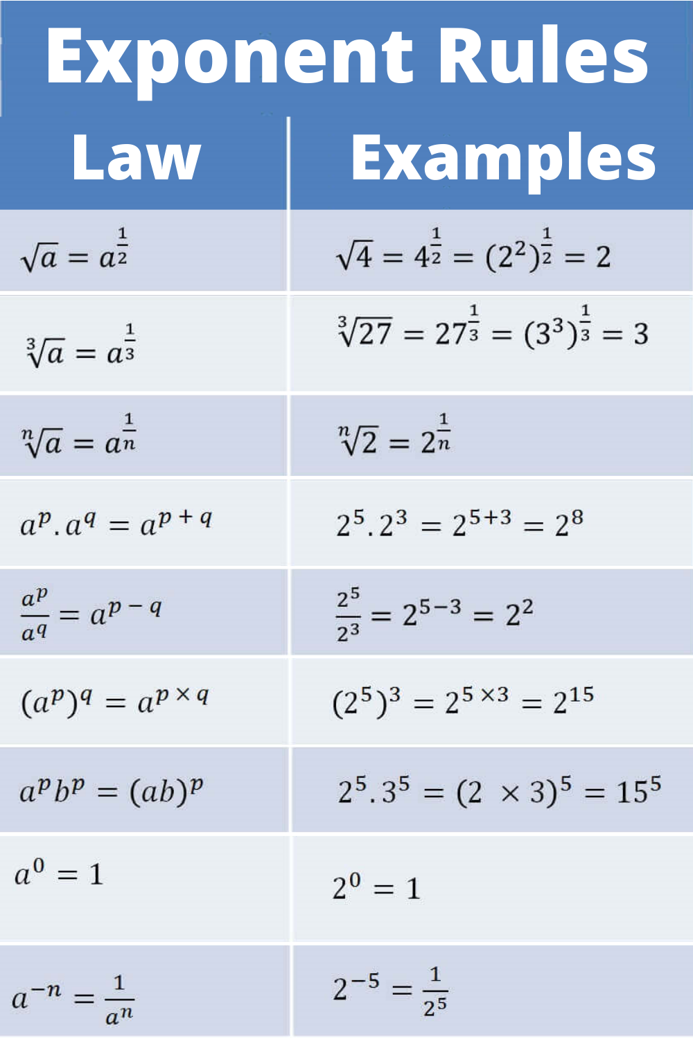
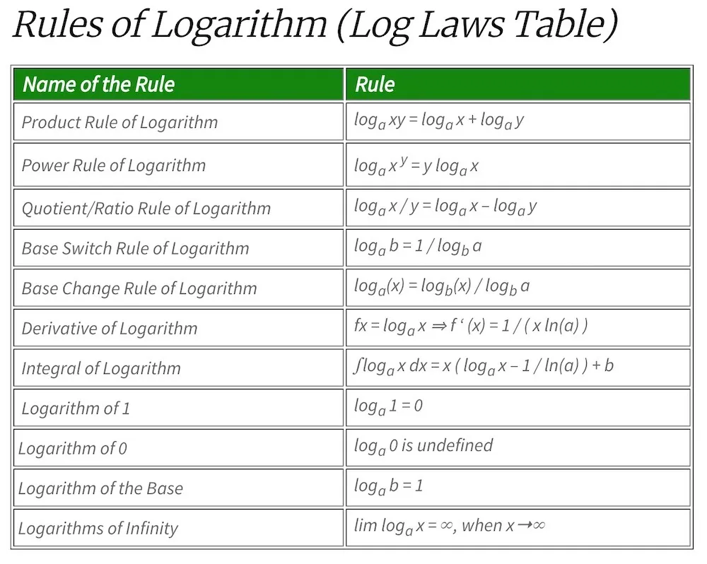
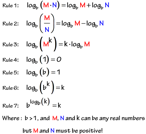
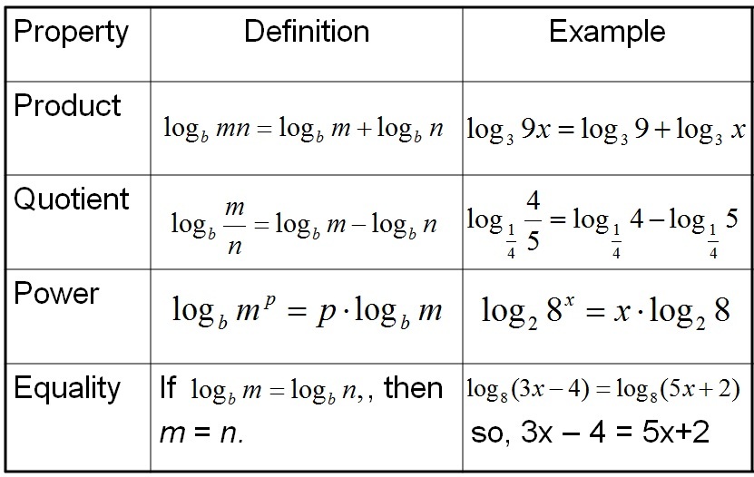
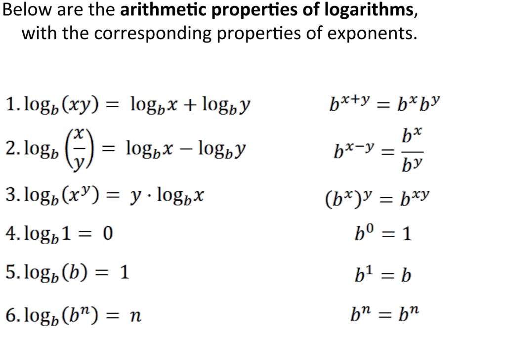
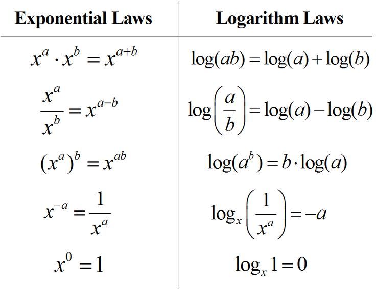
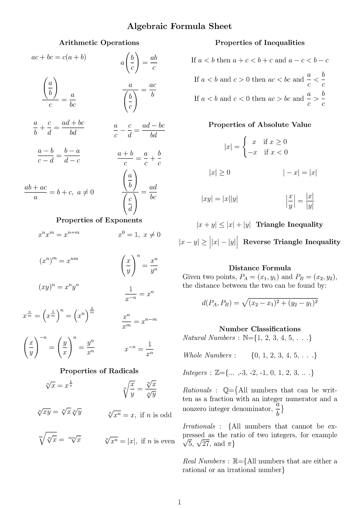
You should have complete mastery of all of these topics:
https://en.wikipedia.org/wiki/Arithmetic
https://en.wikipedia.org/wiki/Logarithm
https://en.wikipedia.org/wiki/Exponentiation
https://en.wikipedia.org/wiki/Nth_root
You should already know the topics outlined here quite well:
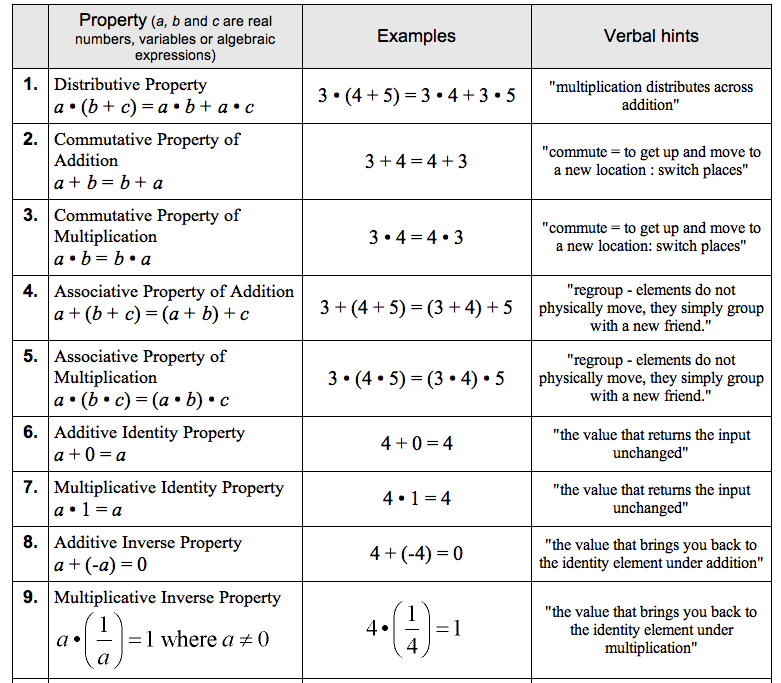
https://en.wikipedia.org/wiki/Elementary_algebra
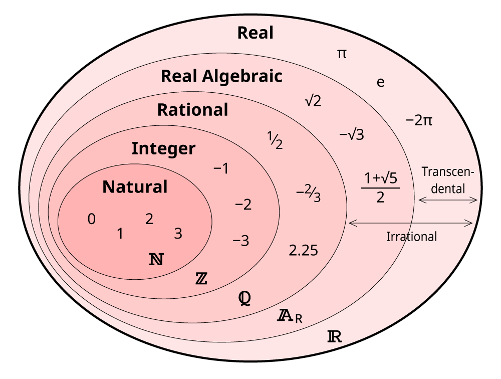
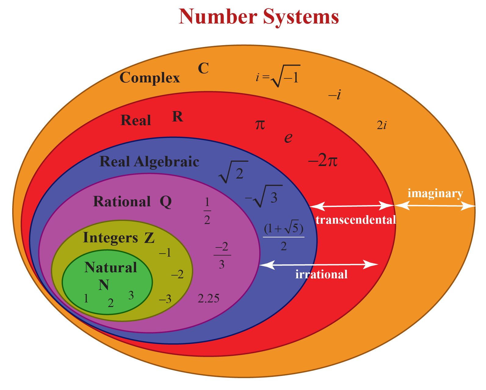
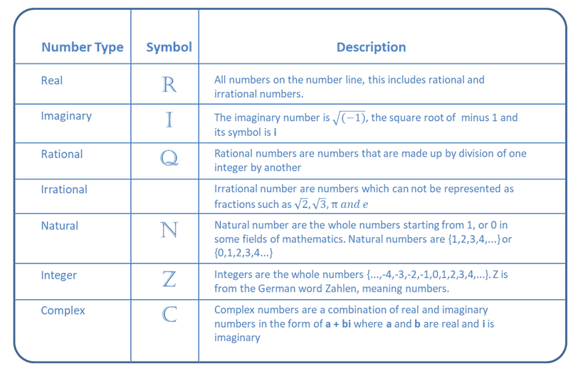
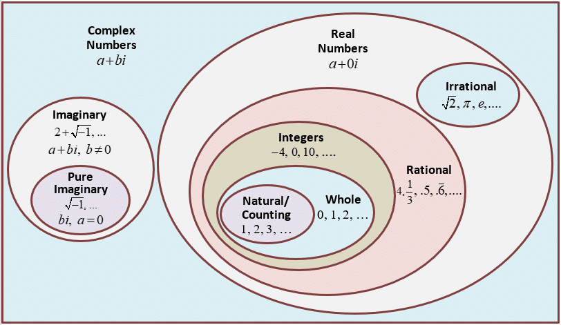
You should be aware of the types of numbers:
https://en.wikipedia.org/wiki/Number
And have a basic understanding of these ideas:
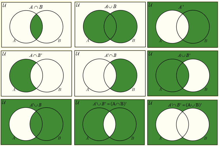
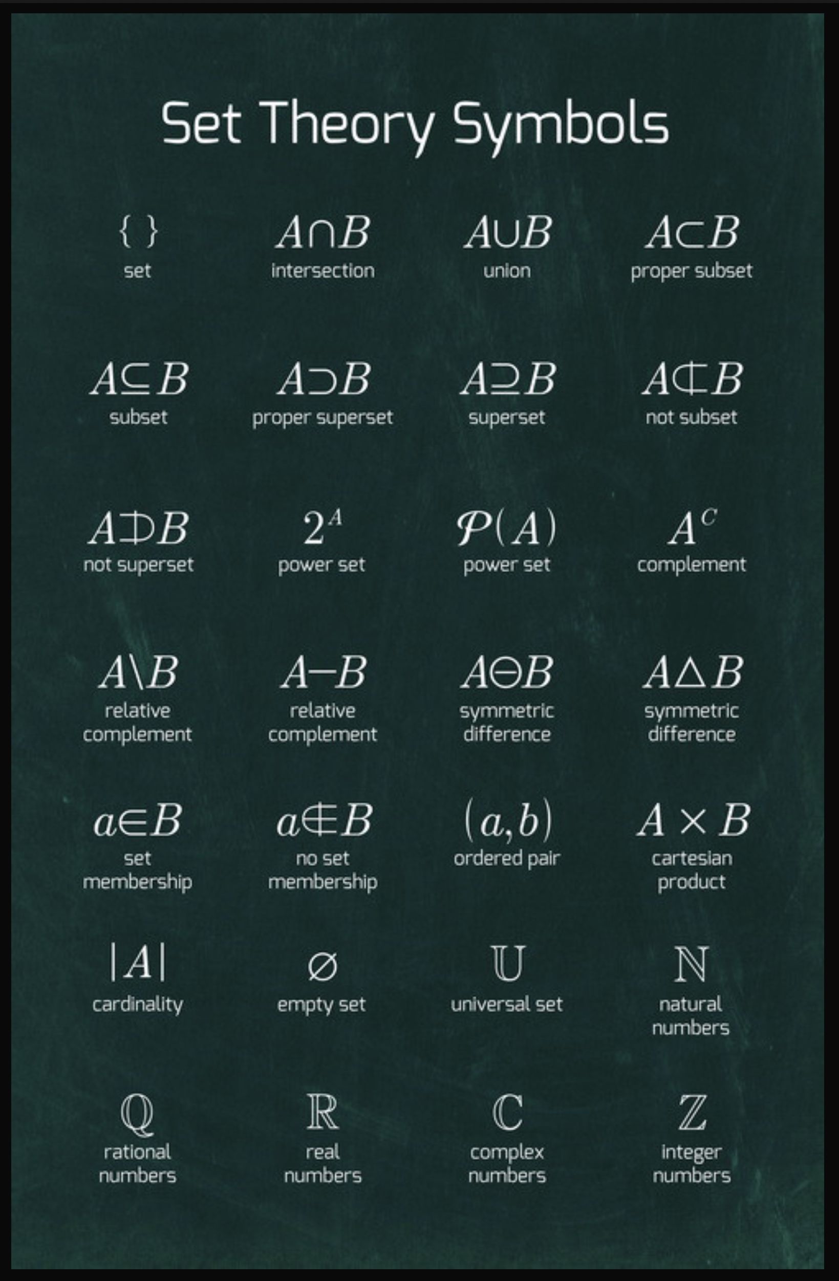
https://en.wikipedia.org/wiki/Set_(mathematics)
https://en.wikipedia.org/wiki/Set_theory
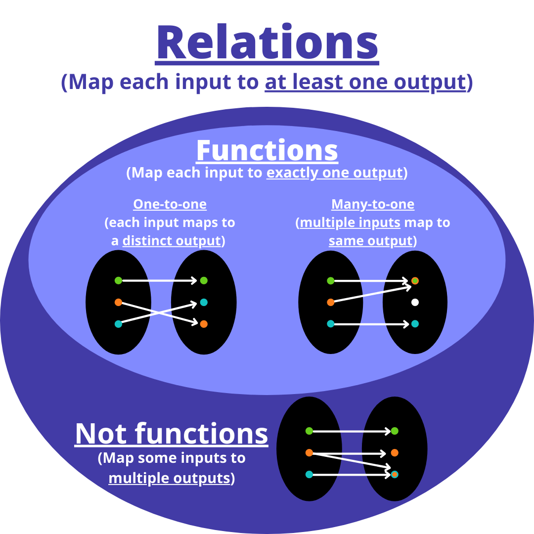
https://en.wikipedia.org/wiki/Function_(mathematics)
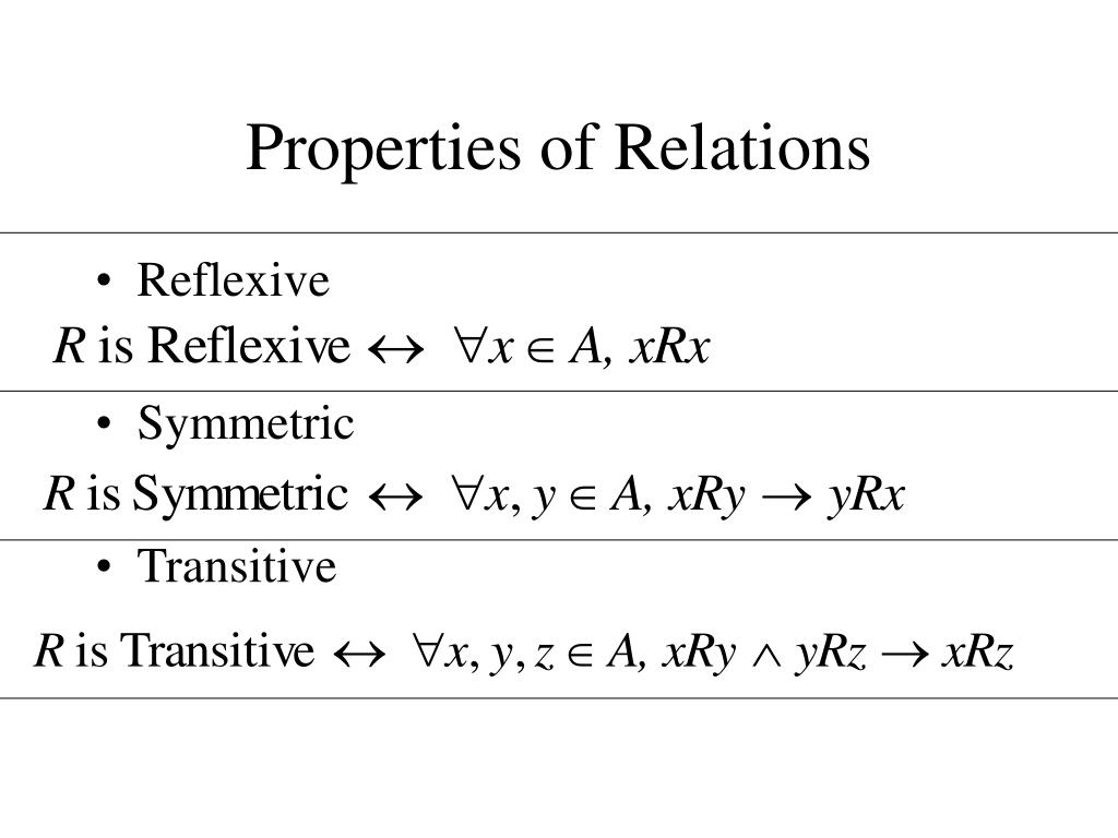
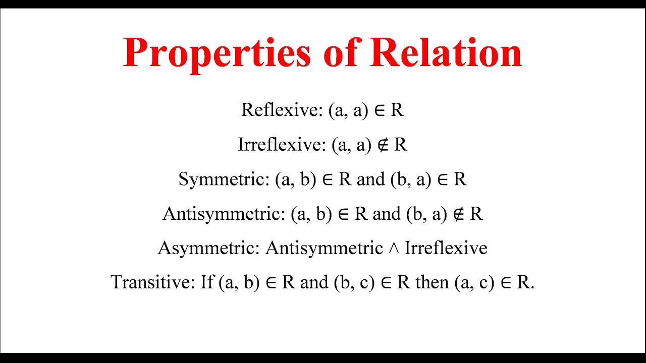
https://en.wikipedia.org/wiki/Relation_(mathematics)
https://wiki.haskell.org/Equational_reasoning_examples
https://www.haskellforall.com/2013/12/equational-reasoning.html
https://www.haskellforall.com/2014/07/equational-reasoning-at-scale.html
https://theory.stanford.edu/~blynn/haskell/eqreason.html
An equation x = y says that x and y have the same value.
Any time you see one of them you can replace it by the other.
Such a replacement is called a substitution.
https://en.wikipedia.org/wiki/Substitution_(logic)#Mathematics
Exactly the same technique can be used to reason about Haskell
programs,
because equations in Haskell are true mathematical equations;
they are not assignment statements.
MathReview/EquationalReasoning.hs
#!/usr/bin/runghc

module EquationalReasoning where

-- Equational reasoning with functions

-- | We can use substitution to reason here:
-- >>> func1 3
-- 5
func1 :: Integer -> Integer
func1 z = 8 - z

-- | We can use substitution to reason using both funcs:
-- >>> func2 3 4
-- 20
func2 :: Integer -> Integer -> Integer
func2 x y = (2 + x) * func1 y

-- Equational reasoning with lists
-- Proofs upcoming in Induction lectures.

xs = [1, 2, 3]

ys = [3, 4, 5]

-- | Theorem 1
-- >>> theoremOne
-- True
theoremOne = length (xs ++ ys) == length xs + length ys

-- This is a function that adds 5 to a number.
f :: Int -> Int
f = (+) 5

-- | This is a home-made version of the `map` in Prelude.
-- >>> myMap f xs
-- [6,7,8]
myMap :: (a -> b) -> [a] -> [b]
myMap _ [] = []
myMap f (x : xs) = f x : myMap f xs

-- The real version is available by default in the default haskell Prelude.
-- https://hackage.haskell.org/package/base-4.21.0.0/docs/Prelude.html#v:map
-- https://hackage.haskell.org/package/ghc-internal-9.1201.0/docs/src/GHC.Internal.Base.html#map

-- | Theorem 2
-- >>> theoremTwo
-- True
theoremTwo = length (map f xs) == length xs

-- | Theorem 3
-- >>> theoremThree
-- True
theoremThree = map f (xs ++ ys) == map f xs ++ map f ys

-- | Theorem 4. See lecture notes for two proofs of this one.
-- >>> theoremFour
-- True
theoremFour = length (map f (xs ++ ys)) == length xs + length ysThe following theorem states an obvious result,
the length of a concatenation,
is the sum of the lengths of the pieces that were concatenated.
This theorem can be proved using list induction (upcoming).
We can use the theorem directly to justify equational reasoning
steps,
and an example is given below.
Let xs, ys :: [a] be arbitrary lists.
Then length (xs ++ ys) == length xs + length ys.
The next theorem says that if you map a function over a list,
the list of results is the same size as the list of arguments.
Let xs :: [a] be an arbitrary list,
and f :: a -> b an arbitrary function.
Then length (map f xs) == length xs.
We also need the following result,
which says that if you map a function over a concatenation of two
lists,
the result could also be obtained by concatenating separate maps over
the original lists.
This theorem is frequently used in parallel functional
programming,
because it shows how to decompose a large problem,
into two smaller ones than can be solved independently.
Let xs, ys :: [a] be arbitrary lists,
and let f :: a -> b be an arbitrary function.
Then map f (xs ++ ys) == map f xs ++ map f ys.
To illustrate how a theorem can be proved using direct equational
reasoning,
we will give a proof for this theorem:
For arbitrary lists xs, ys :: [a],
and arbitrary f :: a -> b,
the following equation holds:
length (map f (xs ++ ys)) == length xs + length ys.
Proof.
We prove the theorem by equational reasoning,
starting with the left hand side of the equation,
and transforming it into the right hand side.
length (map f (xs ++ ys))
  = length (map f xs ++ map f ys)           { map (++) }
  = length (map f xs) + length (map f ys)   { length (++) }
  = length xs + length ys                   { length map }
There are usually many ways to prove a theorem; here is an alternative version:
length (map f (xs ++ ys))
  = length (xs ++ ys)           { length map }
  = length xs + length ys       { length (++) }
Either proof is fine, and you don’t need to give more than one!
It is a matter of taste and opinion as to which proof is better.
Sometimes a shorter proof seems preferable to a longer one,
but issues of clarity and elegance may also affect your choice.
You may be wondering why you haven’t used equational reasoning for
years,
as it is so simple and powerful.
The reason is that equational reasoning requires equations,
which say that two things are equal.
Imperative programming languages simply don’t contain any
equations.
Consider the following code, which might appear in a C or Java
program:
n = n + 1
That might look like an equation, but it isn’t!
It is an assignment.
The meaning of the statement is a command:
“fetch the value of n, then add 1 to it,
then store it in the memory location called n,
discarding the previous value.”
This is not a claim that n has the same value as n + 1.
Because of this, many imperative programming languages use a
distinctive notation for assignments.
For example, Algol and its descendants use the := operator:
n := n + 1
What is different about pure functional programming languages like
Haskell,
is that x = y really is an equation, stating that x and y have the same
value.
Furthermore, Haskell has a property called referential
transparency.
This means that if you have an equation x = y,
then you can replace any occurrence of x by y,
and you can replace any occurrence of y by x.
This is, of course, subject to various restrictions;
you have to be careful about names and scopes,
and grouping with parentheses, etc.
The imperative assignment statement n := n + 1
increases the value of n.
Whereas the Haskell equation n = n + 1 defines n
to be the solution to the mathematical equation.
This equation has no solution, so the result is that n is
undefined.
If the program ever uses an undefined value like n,
then the computer will either give an error message or go into an
infinite loop.
Assignments have to be understood in the context of time passing as a
program executes.
To understand the n := n + 1 assignment,
you need to talk about the old value of the variable, and its new
value.
In contrast, equations are timeless,
as there is no notion of changing the value of a variable.
Indeed, there is something peculiar about the word “variable”.
In mathematics and also in functional programming,
a variable does not vary at all!
To vary means to change over time, and this simply does not
happen.
A mathematical equation like x = 23 means that x has the value 8,
and it will still have that value tomorrow.
If the next chapter says x = 2 + 2,
then this is a completely different variable being defined,
which just happens to have the same name;
it doesn’t mean that 8 shrank over the course of a few pages.
A variable in mathematics means “a name that stands for some
value”,
while a variable in an imperative programming language means
“a memory location whose value is modified by certain
instructions”.
As one would expect, there is a price to be paid for the enormous
benefits of equational reasoning.
Pure functional languages like Haskell, as well as mathematics
itself,
are demanding in that they require you to think through a problem
deeply,
in order to express its solution with equations.
It’s always possible to hack an imperative program,
by sticking an assignment in it somewhere in order to patch up a
problem,
but you cannot do that in a functional program.
On the other hand, if our goal is to build correct and reliable
software,
and this should be our goal,
then the discipline of careful thought will be repaid in higher quality
software!