Note no teacher super-category as I define above.
Previous: 00-Introduction.html
Problems and solvers can, and
should, be distinguished.
Evolutionary computing is primarily concerned with problem
solvers.
To characterize any problem solver,
it is useful to identify the kind of problems to which it can be
applied.
The set of all given problems can be classified in different ways.
These methods are not mutually exclusive.
Any given problems fit in a different category for each of the
below methods.
We will now classify problems several different ways below:
We enumerate these various methods below:
(Classify problems by properties of their solvers)
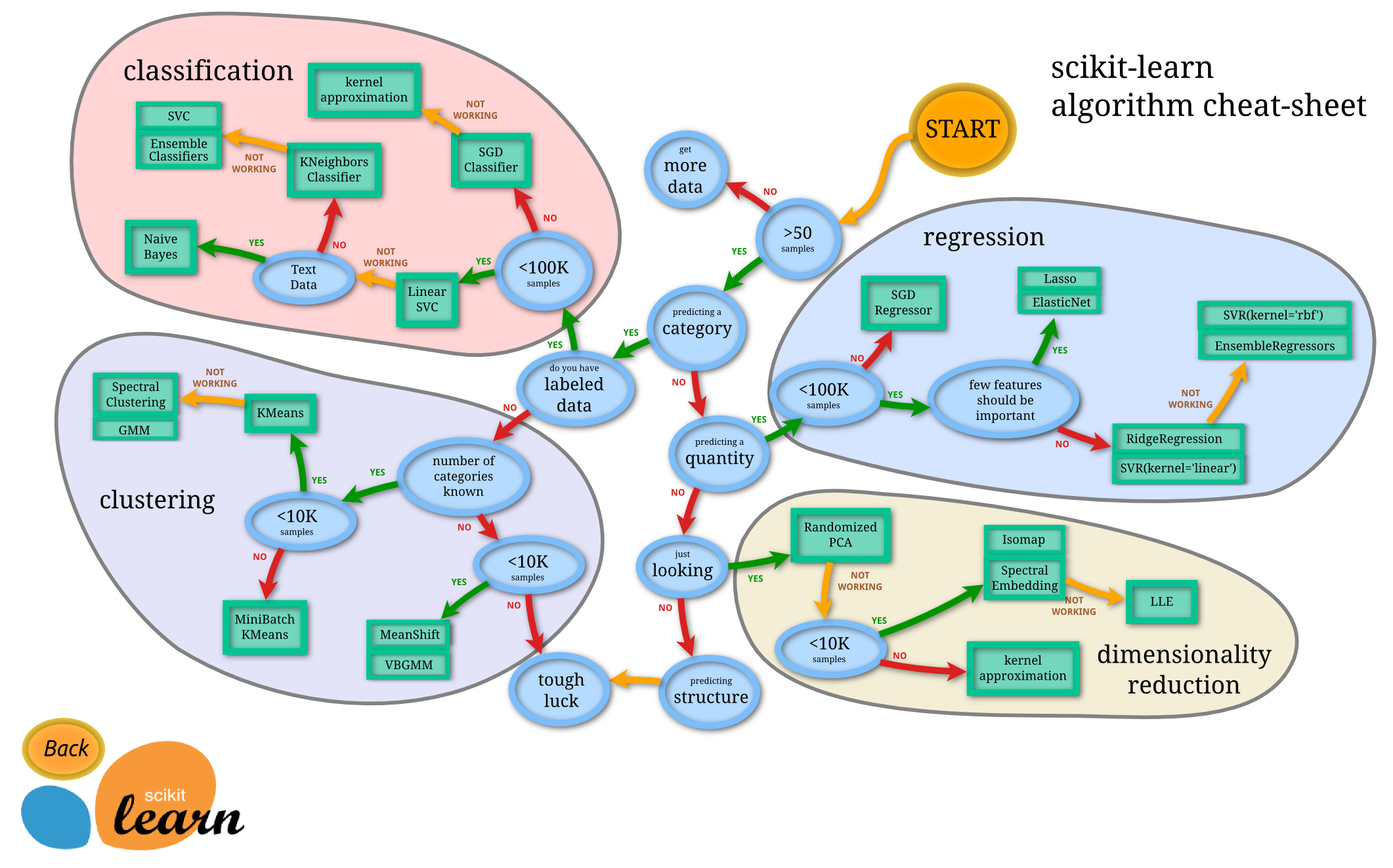
Machine Learning is defined by programs with tuneable
parameters,
that are adjusted automatically, adapting to previously seen data,
so as to improve their behavior.
Machine Learning can be considered a sub-field of Artificial
Intelligence,
since those algorithms can be seen as building blocks,
to make computers learn to behave more intelligently,
by generalizing, rather that just storing and retrieving data
items,
like a database system would do.
AI is just machine learning wrapped into a bot,
or into an autonomous agent with hybrid methods.
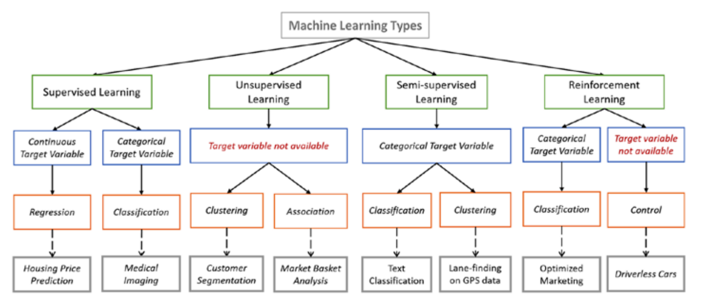
We can separate learning problems in a few large categories by their solvers:
Reinforcement and Supervised:
Lazy neglectful teacher, who just informs you when you win or
lose.
Provides loose, sparse feedback (not really covered in this class).
Micromanaging teaching who tells you every time you act, good/bad,
etc.
The data comes with additional attributes that we want to predict.
Classification:
Samples belong to two or more classes and we want to learn from already
labeled data how to predict the class of unlabeled data.
An example of classification problem would be the handwritten digit
recognition example, in which the aim is to assign each input vector to
one of a finite number of discrete categories.
Another way to think of classification is as a discrete (as opposed to
continuous) form of supervised learning where one has a limited number
of categories and for each of the n samples provided, one is to try to
label them with the correct category or class.
Regression:
if the desired output consists of one or more continuous variables, then
the task is called regression. An example of a regression problem would
be the prediction of the length of a salmon as a function of its age and
weight.
Unsupervised learning
in which the training data consists of a set of input vectors,
x,
without any corresponding target values, y.
The goal in such problems may be:
Clustering:
to discover groups of similar examples within the data,
where it is called clustering, or
Density Estimation:
to determine the distribution of data within the input space.
Dimensionality reduction:
to project the data from a high-dimensional space,
down to two or three dimensions for the purpose of visualization.
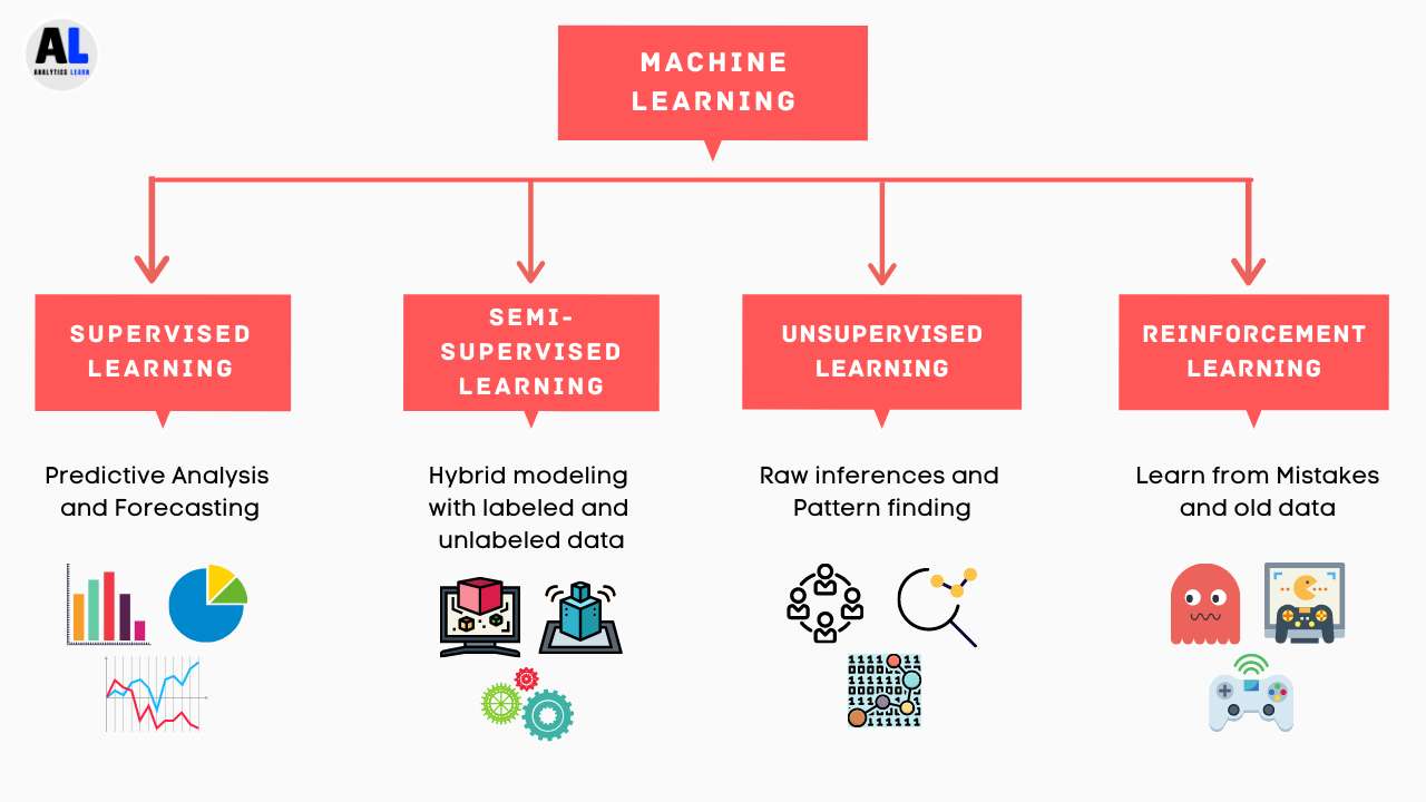
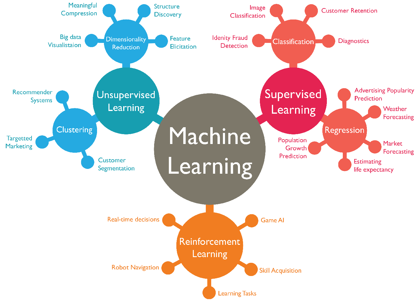
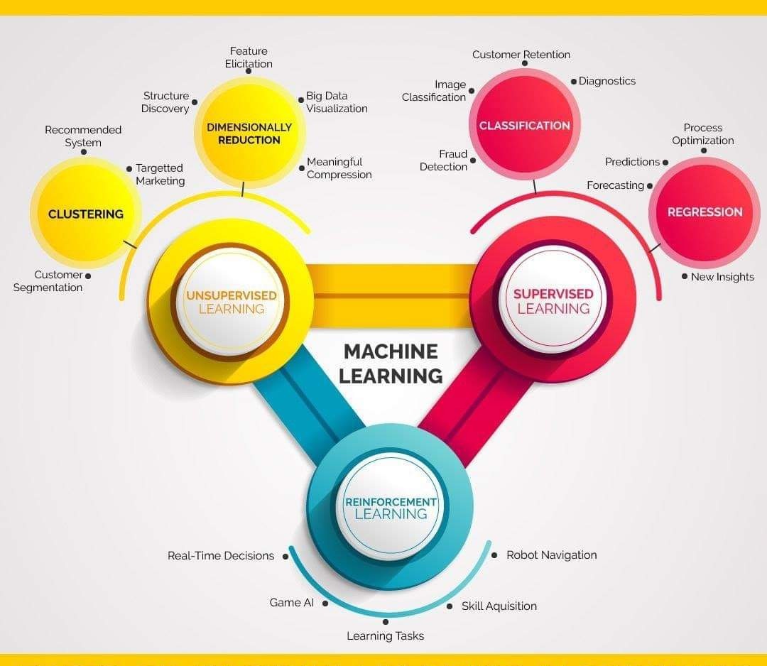
Some other pop ways to classify solvers are depicted below.
Note no teacher super-category as I define above.
Which machine learning method to choose?
Which non-ML method to chose?
Machine learning is a method that solves a sub-set of all problems to
be solved.
For some problems, there are better, simpler methods.
For example, forward-solving an algebraic equation should be done
analytically.
Calculable math is not a machine learning problem!
For some problems, machine learning is a great solution.
This may be a bit too method-centric way to think.
Instead, let’s consider the black-box way of thinking about classifying
these methods.
(classify problems by what is missing in the problem statement)
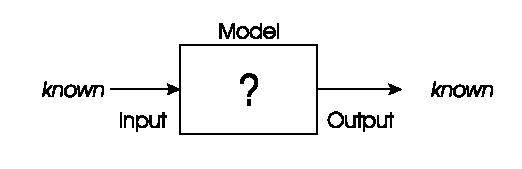
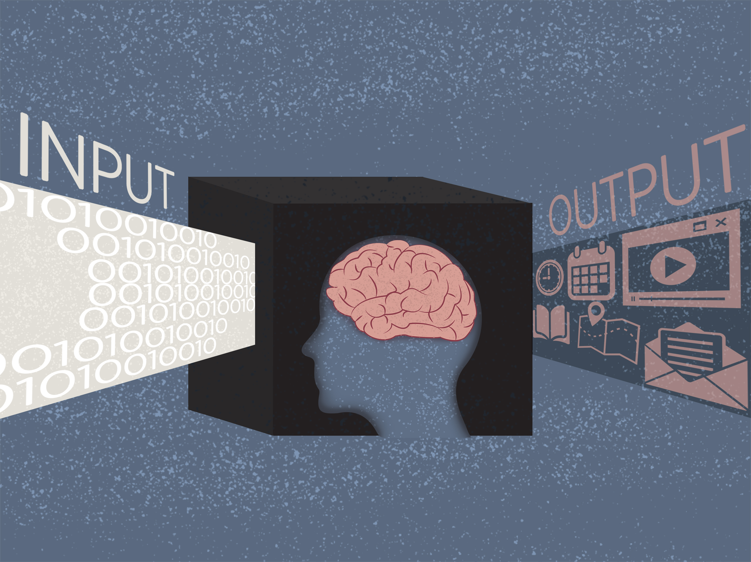
Imagine any computer-based system.
The system initially sits, awaiting some input from either:
a person, a sensor, or another computer.
When input is provided,
the system processes that input through some computational model,
and provides an output.
The model’s details are not specified in general.
Hence the name black box…
The purpose of this model is to represent some aspects of the
world,
relevant to the particular application.
A classic “Black box” model consists of 3 components:
1. input
2. model
3. output
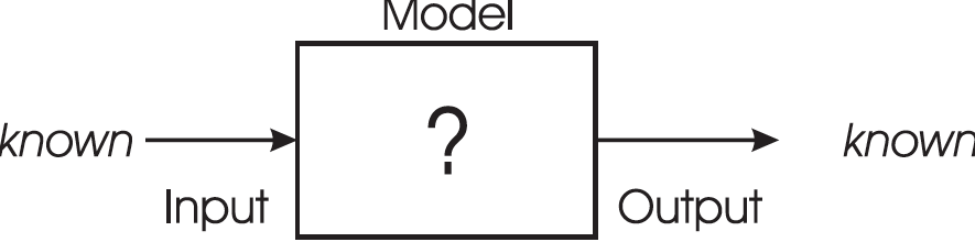
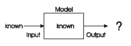
Directionality
This model is like a one-way function in math.
Going forward:
The input and model are known, but the output is not.
It is analytically or easily computable going forward
Going in reverse:
The output is known, and either the input or model are unknown.
It is computationally intractable to compute the process going backward
efficiently.
In reverse, it may be an inverse problem,
or search process through a large set of solutions or models,
going backward from a goal output.
Input:
When designing aircraft wings,
the inputs might represent a description of a proposed wing shape.
Model:
The model might contain equations of complex fluid dynamics,
to estimate the drag and lift coefficients of any wing shape.
Output:
These estimates form the output of the system.
Input:
A voice control system for smart homes takes as input,
the electrical signal produced when a user speaks into a microphone.
Model:
Model maps patterns in electrical wave-forms coming from an audio
input,
onto the outputs that would normally be created by key-presses on a
keyboard.
Output:
Suitable outputs might be commands to be sent to devices:
the heating system, the TV set, or the lights.
One ultimately has to define, determine, generate, or search for all
the parts of the model.
Each type of problem in this category assumes a different phase of model
development, and a different missing part.
Each component that is unknown defines a different problem
type:
1. Optimization - input unknown
2. Modeling - model unknown
3. Simulation - output unknown
In an optimization problem the model is known,
together with the desired output
(or a description of the desired output),
and the task is to find the input(s) leading to a given output.
Known
Model
Desired output
Unknown
Best input in the set of all inputs
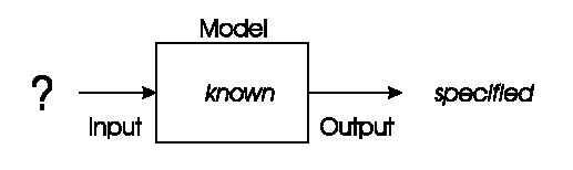
These occur frequently in engineering and design.
The label on the Output reads “specified”, instead of “known”,
because the specific value of the optimum may not be known,
only defined implicitly
(e.g., the lowest numerically of all possibilities).
Examples to cover now:
Traveling salesman problem (TSP)
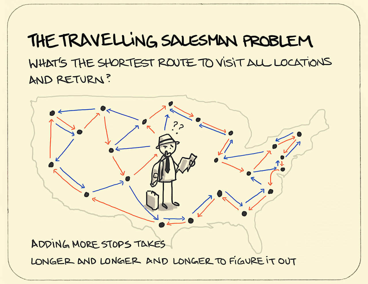
In the abstract version we are given a set of cities,
and have to find the shortest tour which visits each city exactly
once.
For a given instance of this problem, we have:
Input
That for each given sequence of cities (the
inputs),
Model
Uses a formula (the model),
Output
To compute the length of the tour (the output).
The problem is to use a known model to find
an input with a desired output,
that is, a sequence of cities with optimal (minimal) length.
Note that in this example, the desired output is defined
implicitly:
the input in the set of inputs that is the minimum output distance.
Known
Model:
For any given instance, simple formula to add graph edges
Output:
For any given instance, distance of round trip
Unknown
Input:
Best input sequence of cities in the set of all input sequences
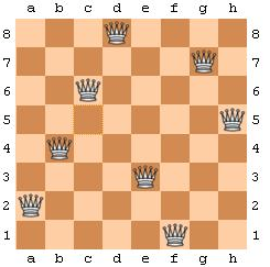
Given an 8-by-8 chessboard and 8 queens,
place the 8 queens on the chessboard without any conflict.
Two queens conflict if they share same row, column or diagonal.
Can be extended to an n queens problem (n>8).
Chess board and eight queens that need to be placed on the board,
in such a way that no two queens can check each other.
They must not share the same row, column, or diagonal.
This problem can be captured by a computational system where:
input is a certain configuration of all eight queens,
model calculates whether the queens in a given configuration check each other or not, and
output is the number of queens not being
checked.
Known
Model:
Simple constraint to check queen conflicts board
Output:
Configuration is valid or not valid (OK/conflict).
Unknown
Input:
A valid board configuration,
from the set of all board configurations
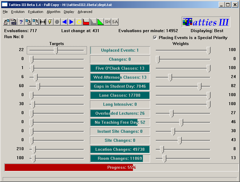
Scheduling is often an enormously big search space.
Timetables must be good.
“Good” is defined by a number of competing criteria.
Timetables must be feasible.
Vast majority of search space is in-feasible.
You may have an intuition for how scheduling is hard:
Out of the set of sub-problem types in scheduling, many are
NP-hard!
* [ ] Exercise (do in class):
Known
Model?
Output?
Unknown
Input?

Known
Model?
Output?
Unknown
Input?
Corresponding sets of inputs and outputs are known,
and a model of the system is sought,
that delivers the correct output,
for each known input
Known
Input
Output
Unknown
Model
We have corresponding sets of inputs and outputs,
and seek a model that delivers correct output,
for every known input:
These occur frequently in data mining and machine learning.
British bank evolved creditability model,
to predict loan paying behavior of new applicants.
Evolving: multiple different prediction models.
Fitness (quality) of the model: model accuracy on historical data.

Known
Input - past financial meta-data for a person.
Output - loan repayment probability (future financial meta-data).
Unknown
Model - predictive formula to compute the creditability from data.
Let us take the stock exchange as an example:
Some economic and societal indices
(e.g., the unemployment rate, gold price, euro–dollar exchange rate,
etc.)
form the input,
and the Dow Jones index is seen as output.
The task is now to find a formula (model),
that links the known inputs to the known outputs,
thereby representing a model of this economic system.
If one can find a correct model for the known data (from the
past),
and if the relationships captured in this model remain true,
then we have a prediction tool for the value of the Dow Jones
index,
given new data in the future.
Known
Input - ?
Output - ?
Unknown
Model - ?
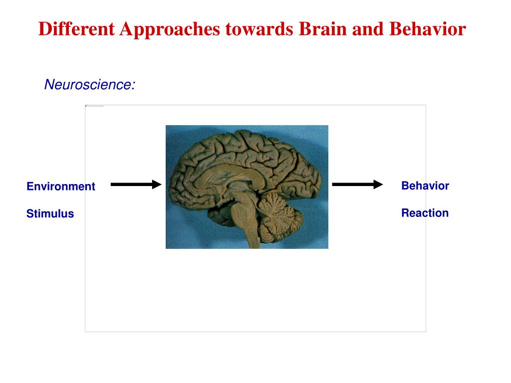
The brain is like a black box:
* [ ] Exercise (do):
Known
Input - ?
Output - ?
Unknown
Model - ?
Problem:
Identifying traffic signs in images,
perhaps from video feeds in a smart car.
System is composed of two elements:
First, in a pre-processing stage,
image processing routines take the electrical signals produced by the
camera,
divide these into regions of interest that might be traffic signs,
and for each one they produce a set of numerical descriptors,
of the size, shape, brightness, contrast, etc.
These values represent the image in a digital form,
and we consider the pre-processing component to be given for now.
Second, in the main black box system:
Input
each input is a vector of numbers describing a possible
sign.
Output
the corresponding output is a label from a predefined
set,
e.g., “stop”, “give-way”, “50”, etc. (the traffic sign).
Model
The model is then an algorithm,
which takes images as input,
and produces categorical labels of traffic signs as output.
Task:
Abstractly, the task goal is to produce a model,
that responds with the appropriate traffic sign labels,
in every possible situation.
In practice, the set of all possible image configurations would be a
sample,
represented by a large collection of images that are all labeled
appropriately.
Then the modeling problem is reduced to finding a model,
that gives a correct output for each image in the collection.
Known
Input
Images of signs represented as vectors.
Output
Sign identity (category) for each input.
Unknown
Model
In theory, model with the minimum output error for all potential
inputs.
In practice, model that minimizes the output error for
all input training data.
wait… isn’t that last thing an optimization problem??
Modeling problems can often be conceptually transformed into optimization problems.
Designate the error rate of a model as either:
the quantity to be minimized, or
its hit rate to be maximized.
Example:
Back to traffic sign identification problem…
This can be formulated as a modeling problem:
Find the best model (m) that maps each one of a
collection of input images onto the appropriate
output label identifying the traffic signs in that
image.
The best model m that solves the problem is unknown in advance
In order to find a solution we need to start by choosing a technology,
maybe:
decision tree,
artificial neural network,
a LISP expression, or
another piece of hacky Python code…
This choice allows us to specify the required form, or syntax of
m.
Having done that, we can define the set of all possible solutions,
M,
for our chosen technology,
being all correct expressions in the given syntax,
e.g.,
all decision trees with the appropriate variables, or
all possible artificial neural networks with a given topology.
Now we can define a related optimization problem:
The set of inputs is M,
and the output for a given m ∈ M,
is an integer saying how many images were correctly labeled by m.
What is a solution of this optimization problem,
with the maximum number of correctly labeled images?
A solution to the original modeling problem.
Known
Input
Images of signs represented as vectors.
Output
Sign identity (category) for each input.
Unknown
Model
Model that minimizes the output error for all input training data.
Known
Model
Evaluation function for the performance of M.
Output
The actual performance of each m in M (error rate).
Unknown
Input
The best input m in the set of all models, M.
Examples include:
Evolutionary machine learning,
Predicting stock exchange,
Voice control system for smart homes.
Conclusion of this transformation exercise:
Optimization and Modeling are both a form of search!
A big question:
Is all learning a form of search?
Mention: No free lunch theorem.
(the easy, often deterministic one, which does not usually require searching)
In a simulation problem,
we know the system model,
and some inputs,
and need to compute the outputs,
corresponding to the inputs:
Assumptions
The existing parts of the black box developed earlier (inputs and
model).
Known
Input
Model
Unknown
Output
We have a given model,
and wish to know the outputs that arise,
under different input conditions
These occur frequently in design,
and in massive real-world manipulations like socioeconomic contexts.
Often used to answer “what-if” questions in evolving dynamic environments:
Here we rely on a big assumption:
The model has already been developed,
merely by manual design,
or perhaps via a process of systematic search (optimization)!
These are cost-reducing measures!
Using a model is much cheaper than building a real system,
and measuring its properties in the physical world!
Cost is not merely a convenient a shortcut.
Often, testing millions of designs is necessary,
and yet building millions of tests may be essentially impossible.
Cost can make-or-break whether engineering a system successfully is even
possible at all!
As an example:
Think of an electronic circuit,
perhaps a filter cutting out low frequencies in a signal.
Assumption
Existing parts of the black box were developed earlier.
We built a model of electrical physics already, at some previous stage
of work.
It is likely pretty good, given the formulaic nature of this system.
Known
Input:
For any given input signal,
the electrical physics model can compute the output signal.
Model:
Our model is a complex system of formulas (equations and
inequalities),
describing the working of the circuit.
Unknown
Output:
The performance of two circuit designs,
which can then be compared.
Benefit:
This is much cheaper than building the circuit,
and measuring its properties in the physical world.
Another example is that of a weather forecast system.
Assumption
Existing parts of the black box were developed earlier.
We built a model of weather dynamics already, at some previous stage of
work.
It may be imperfect, but that’s not the problem we’re dealing with
here.
Known
Input:
Inputs are the meteorological data from previous timepoints,
including:
temperature, wind, humidity, rainfall, etc.,
Model:
The model here is a temporal one,
to predict future meteorological data.
Unknown
Output:
Output data formats are actually the same:
temperature, wind, humidity, rainfall, etc.,
but at a different “future” time.
Testing a hypothetical intervention:
What happens to the economy if you increase interest rates?
Can you test this 1000s of times?
Is it ethical to test?
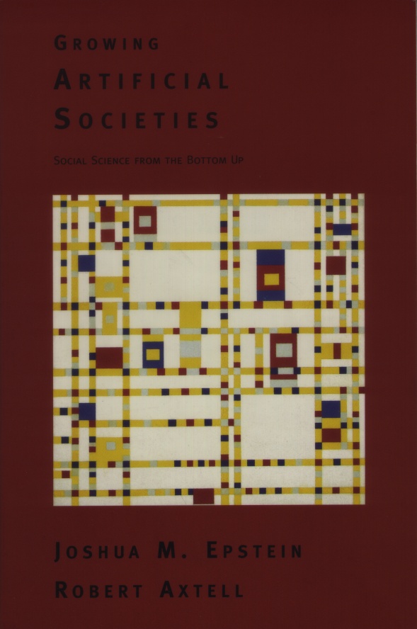
Simulation to determine what would happen in a really big
experiment!
Simulating trade, economic competition, etc. to calibrate models.
Use models to optimize strategies and policies.
Evolutionary economy modeling demonstrates that survival of the fittest is universal (big/small fish).
* [ ] Exercise (do in class):
What happens to the economy if you increase interest rates?
Assumption
Existing parts of the black box developed earlier?
Known
Input - ?
Model - ?
Unknown
Output - ?
Why have sex?
Why do almost all eukaryotes do sexual reproduction?
Does it not seem unnecessarily complicated and expensive?
Biologically, sexual multi-parent reproduction, can make evolution more efficient (and nimble/fast).
Pictures censored…
2 parent:
This is the reason most higher life does sexual reproduction!
Greater than 2 parent:
Does not exist naturally on Earth, in carbon…
However, it kind of does:
Have a mitochondrial disease and want to prevent it while still having
children?
Just head to eastern Europe for a a 3-parent baby.
Mom+Dad’s fertilized autosomes injected into other woman’s egg with it’s
own mitochondrial genome!
Simulations can inform studies of living organisms too:
Incest prevention keeps evolutionary simulations from
degeneration.
(we knew this already…)
The method however makes a more general, grander conclusion:
Inbreeding is bad for evolution, no matter the physical substrate it is
implemented in.
Though surprisingly in both EC and biology,
we observe the benefit is a quantitative continuum,
with both in-breeding and out-breeding depression (more later).
Assumption
Existing parts of the black box developed earlier.
Model of genetic mechanisms, recombination mechanisms, etc.
Known
Input:
Population and fitness.
Model:
Reproduction, recombination, evolution.
Unknown
Output:
New population, and new fitness.
+++++++++++++ Cahoot-01-1
Classify problems by whether they include reverse search or merely forward calculation.
Recall above:
Black box models are usually forward-directional,
one way, and not easily invertible.
Thus, solving a simulation problem is different from solving an optimization or a modeling problem.
In simulation,
we only need to apply the model to some inputs and simply wait for the
outcome.
In optimization or a modeling,
we require the identification of a particular object in a space of
possibilities.
This search space can be, and usually is, enormous.
The process of problem solving can be viewed as search,
through a potentially huge set of possibilities,
to find the desired solution.
The problems that are to be solved this way can be seen as search
problems.
https://en.wikipedia.org/wiki/Artificial_intelligence#Search_and_optimization
Define: Search space
Collection of all objects of interest including the desired
solution.
For optimization problems,
such a definition can be explicit,
e.g., a board configuration where the number of checked queens is zero,
or implicit,
e.g., a tour that is the shortest of all tours.
For modeling problems,
a solution is defined by the property that it produces the correct
output for every input.
In practice, however, this is often relaxed,
only requiring that the number of inputs for which the output is correct
be maximal.
This approach transforms the modeling problem into an optimization
one.
Benefit of classifying these problems as
search:
Search spaces are big!
How large is the search space for different tours through n
cities in the TSP?
Such search spaces can indeed be very large;
for instance, the number of different tours through n cities is (n −
1)!
In classification modeling,
the number of decision trees with real-valued parameters is
infinite!
We can study solvers as independent, generalizable
methods,
for searching through spaces more efficiently.
+++++++++++++ Cahoot-01-2
Discussion question:
How generally can we assert that problem solving is just an instance of search?
Classify by whether they are categorical, or numerical, discrete or continuous.
“Every task involves constraint,
Solve the thing without complaint;
There are magic links and chains,
Forged to loose our rigid brains.
Structures, strictures, though they bind,
Strangely liberate the mind.”
- James Falen
https://en.wikipedia.org/wiki/Mathematical_optimization
https://en.wikipedia.org/wiki/Constraint_satisfaction
Defines a way of assigning a value to a possible solution that reflects its quality on numerical scale.
Examples:
Length of a tour visiting given set of cities (to minimize).
Number of un-checked queens (to maximize).
Number of images in a collection that are labeled correctly,
by a given model m (to maximize).
A binary evaluation telling whether or not a given requirement holds.
Examples:
A sequence of cities (a tour),
where city X is visited after city Y.
A configuration of eight queens on a chessboard,
such that no two queens check each other
| Constraints | Objective function | |
|---|---|---|
| - | Yes | No |
| Yes | Constrained optimisation problem | Constraint satisfaction problem |
| No | Free optimisation problem | No problem |
Free Optimization Problem (FOP) - numerical
Numerical optimization - continuous, real numbers
Combination optimization - discrete numbers (Boolean, integers)
Constraint satisfaction Problem (CSP) - categorical
Constrained Optimization Problem (COP) - both numerical and categorical
Do they all fit only in one category?
Transformations
Categorical constraint problems can often be transformed into
optimization problems.
The trick is like transforming modeling problems into optimization
problems.
Rather than requiring perfection, we just:
count the number of satisfied constraints,
(e.g., non-checking pairs of queens),
and introduce this as an objective function to be maximized.
Obviously, an object (e.g., a board configuration),
is a solution of the original constraint satisfaction problem,
if and only if, it is a solution of this associated optimization
problem.
How can we formulate the 8-queens problem in to a FOP/CSP/COP?
Define search space S,
to be the set of all board configurations with eight queens.
Objective function (f),
which reports the number of free queens,
for a given configuration.
Define a valid solution is any configuration of s ∈ S,
with number of free queens maximized,
i.e., f(s)=8.
Define same search space S,
to be the set of all board configurations, s.
Define a constraint function, φ,
such that φ(s)=true,
if and only if, no two queens check each other,
for a given configuration, s.
Valid solution is any configuration, s,
where the constraint is met.
In any solution of the eight-queens problem,
the number of queens in each row and column must be exactly one.
Distinguish:
Vertical and and horizontal constraints (for row attack).
It is easy to find configurations with one queen in each column and in
each row.
Diagonal constraints (for diagonal attack).
It may be a little harder to implement the diagonal.
Rather than constrain all 3 at once.
Valid row, col configurations are taken as a subset of the original
search space.
Let us define the subset containing only the valid row, col as S’
New COP is defined over original S,
with a modified constraint, ψ’,
such that ψ’(s)=true,
if and only if both:
All vertical and horizontal constraints are satisfied in s.
i.e. φ’(s)=true if and only if s is in S’
A new function g,
that reports the number of pairs of queens in s,
that violate the diagonal constraints.
A board configuration is a solution of the eight-queens
problem,
if and only if,
it is a solution of this constrained optimization problem with
both:
φ’(s) = true
g(s) = 0
Why do these three formulations matter?
Problem encoding has a huge impact on learning in EC!
+++++++++++++ Cahoot-01-3
Classify by their computational complexity:
Resource utilization as a function of input size.
First, we talked about classes of problem by solver.
Then, we only looked at classifying the problem itself, not problem
solvers.
Now, complexity classification scheme needs the properties of the
problem solver.
Benefit of this scheme:
These methods make it possible to define and quantify the difficulty of
a computational problem.
Problem size:
Dimensionality of the problem at hand,
and number of different values for the problem variables.
Running-time:
Resource utilization (time, memory, joules) the algorithm takes to
terminate.
As a function of problem size, we make proofs about the:
upper, lower, or upper and lower bound on either:
Worst-case, Best case, or Average case resource utilization,
Examples:
Polynomial, super-polynomial, exponential
Problem reduction:
Transforming current problem into another,
via mapping is sometimes provably possible.
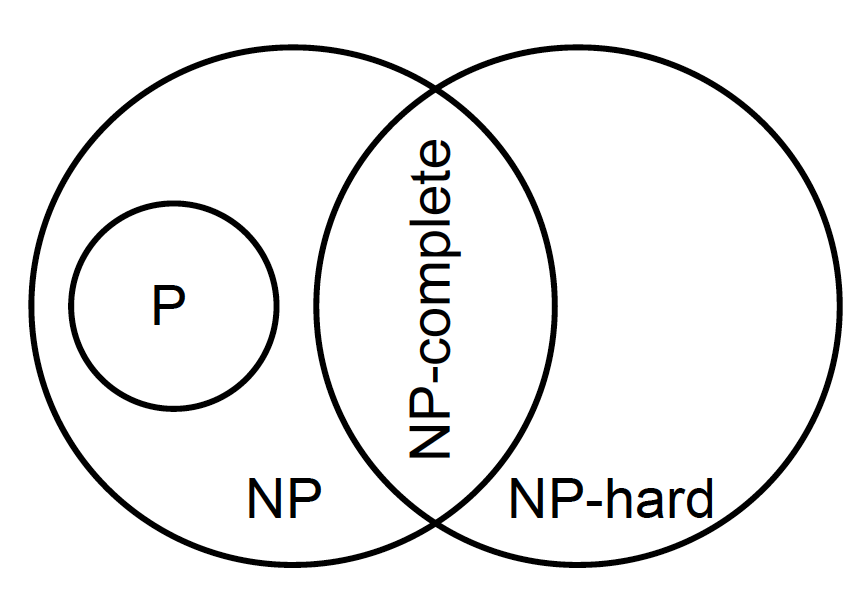
The difficulty of a problem can now be classified:
Class P:
algorithm can solve the problem in polynomial time, and
worst-case running-time, for problem size n, is less than F(n),
for some polynomial formula F.
Class NP:
problem can be solved (no statement about run-time), and
any solution can be verified within polynomial time by some other
algorithm.
P is subset of NP.
Class NP-complete:
problem belongs to class NP (meets those criteria), and
any other problem in NP can be reduced to this problem,
by an algorithm running in polynomial time.
Class NP-hard:
problem is at least as hard as any other problem in NP-complete,
but
solution cannot necessarily be verified within polynomial time.
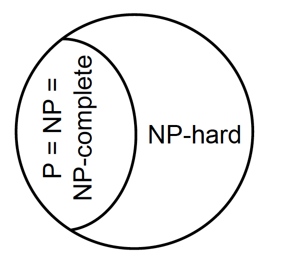
P is provably different from NP-hard.
Not proven whether P is always different from NP.
For now: use of approximation algorithms and meta-heuristics.
The Million dollar problem (prize money)
Image below: P≠NP (left) versus P=NP (right)
For more
https://en.wikipedia.org/wiki/Computational_complexity
https://en.wikipedia.org/wiki/Asymptotic_computational_complexity
M.Garey and D.Johnson. Computers and Intractability.
A Guide to the Theory of NP-Completeness.
Freemann, San Francisco, 1979.
A classic book explaining the concepts of NP-Completeness and problem
difficulty.
C.M. Papadimitriou.Computational Complexity.
Addison-Wesley, Reading, Massachusetts, 1994
C.M. Papadimitriou and K.Steiglitz.
Combinatorial Optimization: Algorithms and Complexity.
Prentice Hall, Englewood Cliffs, NJ, 1982.
Two more good books describing the theory of what makes problems
hard.
F. Neumann and C.~Witt.
Bioinspired Computation in Combinatorial Optimization: Algorithms and
Their Computational Complexity.
Springer, Natural Computing Series, 2010.
Relates bio-inspired algorithms such as evolutionary algorithms to
computational complexity