
Can we optimally vary parameters over the run?
An EA has many strategy parameters, e.g.
Good parameter values facilitate good performance.
Q1: How to find good parameter values?
EA parameters are rigid (constant during a run).
But, an EA is a dynamic, adaptive process.
Thus, optimal parameter values may vary during a run.
Q2: How to vary parameter values?
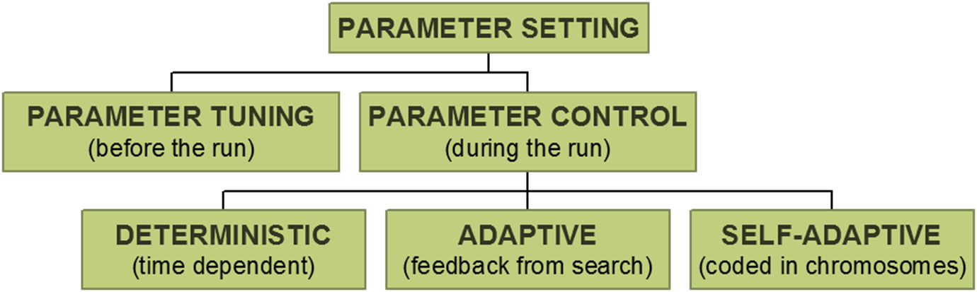
Parameter tuning:
the traditional way of testing and comparing different values before the
“real” run.
Problems:
Parameter control:
setting values on-line, during the actual run , e.g.
Problems:
* finding optimal p is hard, finding optimal p(t) is harder
* still user-defined feedback mechanism, how to “optimize”?
* when would natural selection work for strategy parameters?
We’ve covered some of these previously:
Assign a personal W to each individual
Incorporate this W into the chromosome: (x1, …,
xn, W)
Apply variation operators to xi’s and W
Alert:
val((x, W)) = f(x) + W × penalty(x)
while for mutation step sizes we had
eval((x, σ))= f(x)
this option is thus sensitive “cheating” ⇒ makes no sense
However, one could use an objective tournament to evaluate
fitness,
and still evolve the fitness function.
Various forms of parameter control discussed above can be distinguished by:
| σ(t) = 1-0.9*t/T | σ’ = σ/c, if r > ⅕ … | (x1, …, xn, σ) | (x1, …, xn, σ1, …, σn) | W(t) = (C*t)α | W’=β*W, if bi∈F | (x1, …, xn, W) | |
|---|---|---|---|---|---|---|---|
| What | Step size | Step size | Step size | Step size | Penalty weight | Penalty weight | Penalty weight |
| How | Deterministic | Adaptive | Self-adaptive | Self-adaptive | Deterministic | Adaptive | Self-adaptive |
| Evidence | Time | Successful mutations rate | (Fitness) | (Fitness) | Time | Constraint satisfaction history | (Fitness) |
| Scope | Population | Population | Individual | Gene | Population | Population | Individual |
What is changed?
Practically any EA component can be parameterized,
and thus controlled on-the-fly:
Note that each component can be parameterized,
and that the number of parameters is not clearly defined.
Despite the somewhat arbitrary character of this list of
components,
and of the list of parameters of each component,
we will maintain the ‘what-aspect’ as one of the main classification
features,
since this allows us to locate where a specific mechanism has its
effect.
How are changes made?
Three major types of parameter control:
some rule modifies strategy parameter without feedback from the
search,
based on some counter)
feedback rule based on some measure monitoring search progress
parameter values evolve along with solutions;
encoded into chromosomes, and they undergo variation and selection
The parameter may take effect on different levels:
Note: given component (parameter) determines possibilities
Thus: scope/level is a derived or secondary feature in the classification scheme
Combinations of types and evidences
* Possible: +
* Impossible: -

Of each “What”?
L.D. Whitley, K.E. Mathias, and P. Fitzhorn.
Delta coding: An iterative search strategy for genetic
algorithms,.
In Belew and Booker [46], pages 77–84.
We illustrate variable representations with the delta coding
algorithm of Mathias and Whitley,
which effectively modifies the encoding of the function
parameters.
The motivation behind this algorithm is to:
maintain a good balance between fast search and sustaining
diversity.
In our taxonomy, it can be categorised as an adaptive adjustment of the
representation,
based on absolute evidence.
The GA is used with multiple restarts;
the first run is used to find an interim solution,
and subsequent runs decode the genes as distances (delta values) from
the last interim solution.
This way each restart forms a new hypercube,
with the interim solution at its origin.
The resolution of the delta values can also be altered at the
restarts,
to expand or contract the search space.
Population density can be measured,
by the Hamming distance between the best and worst strings of the
current population.
The restarts are triggered when population diversity
is not greater than 1.
The sketch of the algorithm showing the main idea is given below.
Note that the number of bits for δ can be increased if the same solution
INTERIM is found.
BEGIN
    /* given a starting population and genotype-phenotype encoding */
    WHILE (HD > 1) DO
        RUN GA with k bits per object variable;
    OD
    REPEAT UNTIL (global termination is satisfied) DO
        save best solution as INTERIM;
        reinitialise population with new coding;
        /* k-1 bits as the distance δ to the object value in */
        /* INTERIM and one sign bit */
        WHILE (HD > 1) DO
            RUN GA with this encoding;
        OD
    OD
ENDA.E. Eiben and J.K. van der Hauw.
Solving 3-SAT with adaptive genetic algorithms.
In ICEC-97 [231], pages 81–86.
Evaluation functions are typically not varied in an EA,
because they are often considered as part of the problem to be
solved,
and not as part of the problem-solving algorithm.
In fact, an evaluation function forms the bridge between the two,
so both views are at least partially true.
In many EAs, the evaluation function is derived from the (optimization)
problem at hand,
with a simple transformation of the objective function.
In the class of constraint satisfaction problems, however,
there is no objective function in the problem definition.
One possible approach here is based on penalties.
Let us assume that we have m constraints ci(i ∈ {1, . . . ,
m})
and n variables vj(j ∈ {1, . . . , n}) with the same domain
S.
Then the penalties can be defined as follows:
\(f(\bar{s}) = \sum_{i=1}^m \chi (\bar{s},
c_i),\)
where wi is the weight associated with violating
ci, and
\(\chi(\bar{s}, c_i) = \left\{
\begin{array}{cc} 1 & if\ \bar{s}\ violated\ c_i, \\ 0 &
otherwise. \\ \end{array} \right\}\)
Obviously, the setting of these weights has a large impact on the EA
performance,
and ideally wi should reflect how hard ci is to
satisfy.
The problem is that:
finding the appropriate weights requires much insight into the given
problem instance,
and therefore it might not be practicable.
The step-wise adaptation of weights (SAW) mechanism,
introduced by Eiben and van der Hauw,
provides a simple and effective way to set these weights.
The basic idea behind the SAW mechanism is that,
constraints that are not satisfied after a certain number of steps
(fitness evaluations),
must be difficult, and thus must be given a high weight (penalty).
SAW-ing changes the evaluation function adaptively in an EA,
by periodically checking the best individual in the population,
and raising the weights of those constraints this individual
violates.
Then the run continues with the new evaluation function.
A nice feature of SAW-ing is that:
it liberates the user from seeking good weight settings,
thereby eliminating a possible source of error.
Furthermore, the used weights reflect the difficulty of
constraints,
for the given algorithm, on the given problem instance,
in the given stage of the search.
This property is also valuable since, in principle,
different weights could be appropriate for different algorithms.
Oliver Kramer.
Evolutionary self-adaptation: a survey of operators and strategy
parameters.
Evolutionary Intelligence, 3(2):51–65, 2010.
A large majority of work on adapting or self-adapting EA parameters
concerns variation operators:
mutation and recombination (crossover).
The 1/5 rule of Rechenberg we discussed earlier,
constitutes a classic example for adaptive mutation step size control in
ES.
Furthermore, self-adaptive control of mutation step sizes is traditional
in ES
L. Davis, editor.
Handbook of Genetic Algorithms.
Van Nostrand Reinhold, 1991.
The classic example for adapting crossover rates in GAs is Davis’s
adaptive operator fitness.
The method adapts the rates of crossover operators,
by rewarding those that are successful in creating better
offspring.
This reward is diminishingly propagated back to operators of a few
generations back,
who helped set it all up;
the reward is an increase in probability at the cost of other
operators.
The GA using this method applies several crossover operators
simultaneously,
within the same generation, each having its own crossover rate
pc(opi).
Additionally, each operator has its local delta value,
di,
that represents the strength of the operator,
measured by the advantage of a child created by using that
operator,
with respect to the best individual in the population.
The local deltas are updated after every use of operator i.
The adaptation mechanism recalculates the crossover rates
periodically,
redistributing 15% of the probabilities biased by the accumulated
operator strengths,
that is, the local deltas.
To this end, these di values are normalized,
so that their sum equals 15, yielding dnormi for
each i.
Then the new value for each pc(opi) is 85% of its
old value, and its normalized strength:
\(p_c(op_i) = 0.85 \cdot p_c(op_i) + d^{norm}_i\)
Clearly, this method is adaptive based on relative evidence.
S.W. Mahfoud.
Boltzmann selection.
In Bäck et al., pages C2.5:1–4.
T. Bäck, D.B. Fogel, and Z. Michalewicz, editors.
Handbook of Evolutionary Computation.
Institute of Physics Publishing, Bristol, and Oxford University
Press, New York, 1997.
https://en.wikipedia.org/wiki/Simulated_annealing
J. Arabas, Z. Michalewicz, and J. Mulawka. GAVaPS – a genetic
algorithm
with varying population size. In ICEC-94 [229], pages 73–78.
Z. Michalewicz. Genetic Algorithms + Data Structures = Evolution
Programs.
Springer, 3rd edition, 1996.
T. Bäck.
U. The interaction of mutation rate, selection and self-adaptation
within a genetic algorithm.
V. In Männer and Manderick [282], pages 85–94.
T. Bäck, A.E. Eiben, and N.A.L. van der Vaart.
U. An empirical study on GAs “without parameters”.
V. In Schoenauer et al. [368], pages 315–324.
Tuning works, and increases the search space.
Control works, and increases it further.
Be systematic in both approaches!