https://en.wikipedia.org/wiki/Mathematical_optimization
https://en.wikipedia.org/wiki/Loss_function
https://en.wikipedia.org/wiki/Vector_optimization
https://en.wikipedia.org/wiki/Multi-objective_optimization
A loss function or cost function (sometimes also called an error
function),
is a function that maps an event or values of one or more variables onto
a real number,
representing some “cost” associated with the event.
An optimization problem seeks to minimize a loss function.
An objective function is either a loss function or its opposite
in which case it is to be maximized.
In other specific domains, it is variously called:
a reward function, a profit function, a utility function, a fitness
function, etc.
In EC, we often call this function the fitness function.
A multi-objective optimization attempts to satisfy multiple objective
functions.
It can be formulated as:
\(\min_{x \in X}(f_{1}(x), f_{2}(x), \ldots,
f_{k}(x))\)
where:
the integer \(k \geq 2\) is the number
of objectives,
the set X is the feasible set of decision vectors,
which is typically \(X \subseteq \mathbb
{R}^{n}\),
but it depends on the n-dimensional application domain.
The feasible set is typically defined by some constraint
functions.
In addition, the vector-valued objective function is often defined
as:
\({\begin{aligned}f:X&\to \mathbb {R} ^{k}\\x&\mapsto {\begin{pmatrix}f_{1}(x)\\\vdots \\f_{k}(x)\end{pmatrix}}\end{aligned}}\)
If some objective function is to be maximized,
then it is equivalent to minimize its negative or its inverse.
Many problems contain a number of n possibly conflicting
objectives:
buying a car: speed vs. price vs. reliability,
engineering design: lightness vs. strength.
We have made free use of analogies such as adaptive landscapes,
under the assumption that the goal of the EA in an optimisation
problem,
is to find a single solution that maximises a fitness value,
that is directly related to a single underlying measure of quality.
We also discussed a number of modifications to EAs,
that are aimed at preserving diversity,
so that a set of solutions is maintained;
these represent niches of high fitness,
but we have still maintained the conceptual link to an adaptive
landscape,
defined via the assignment of a single quality metric (objective),
to each of the set of possible solutions.
The quality of a solution may be defined,
by its performance toward possibly conflicting, objectives.
Many applications that have traditionally been tackled,
by defining a single objective function (quality function),
have at their heart a multiobjective problem,
that has been transformed into a single-objective function,
in order to make optimisation tractable.
To give a simple illustration, imagine that we have moved to a new
city,
and are in the process of looking for a house to buy.
There are a number of factors that we will probably wish to take into
account, such as:
number of rooms, style of architecture, commuting distance to work and
method,
provision of local amenities, access to pleasant countryside, and of
course, price.
Many of these factors work against each other (particularly
price),
and so the final decision will almost inevitably involve a
compromise,
based on trading off the house’s rating on different factors.
The example we have just presented is a particularly subjective
one,
with some factors that are hard to quantify numerically.
It does exhibit a feature that is common to multiobjective
problems,
namely that it is desirable to present the user with a diverse set of
possible solutions,
representing a range of different trade-offs between objectives.
The alternative is to assign a numerical quality function to each
objective,
and then combine these scores into a single fitness score,
using some (usually fixed) weighting.
https://en.wikipedia.org/wiki/Multi-objective_optimization#Scalarizing
This approach, often called scalarisation, has been used for
many years,
within the operations research and heuristic optimisation
communities,
but suffers from a number of drawbacks:
The use of a weighting function implicitly assumes that:
we can capture all of the user’s (or problem’s) preferences,
even before we know what range of possible solutions exist.
For applications where we are repeatedly solving different instances
of the same problem,
the use of a weighting function assumes that the weighted preferences
remain static,
unless we explicitly seek a new weighting every time.
Optimisation methods should simultaneously find a diverse set of high-quality solutions.
In multi-objective optimization,
a single solution may not minimize all objective functions
simultaneously.
Therefore, attention is paid to Pareto optimal solutions;
that is, solutions that cannot be improved in any of the
objectives,
without degrading at least one of the other objectives.
Afeasible solution \(x_{1} \in X\) is
said to (Pareto) dominate another solution \(x_{2} \in X\), if
\(\forall i \in \{1,\dots, k\}, f_{i}(x_{1})
\leq f_{i}(x_{2})\), and
\(\exists i \in \{1,\dots, k\}, f_{i}(x_{1})
< f_{i}(x_{2})\).
A solution \(x^{*} \in X\) (and the
corresponding outcome \(f(x^{*})\) is
called Pareto optimal,
if there does not exist another solution that dominates it.
The set of Pareto optimal outcomes, denoted \(X^{*}\),
is often called the Pareto front, Pareto frontier, or Pareto
boundary.
The concept of dominance is a simple one:
given two solutions, both of which have scores according to some set of
objective values
(which, without loss of generality, we will assume to be
maximized),
one solution is said to dominate the other,
if its score is at least as high for all objectives,
and is strictly higher for at least one.
We can represent the scores that a solution A gets,
for n objectives as an n-dimensional vector \(\bar{a}\).
Using the \(\succeq\) symbol to
indicate domination,
we can define \(A \succeq B\) formally
as:
\(A \succeq \iff \forall_i \in {1,...,n} a_i \geq b_i, and \exists_i \in {i,...,n}, a_i > b_i\)
For conflicting objectives, there exists no single solution that
dominates all others,
and we will call a solution nondominated, if it is not dominated by any
other.
All nondominated solutions possess the attribute that,
their quality cannot be increased with respect to any of the objective
functions,
without detrimentally affecting one of the others.
Such solutions usually lie on the edge of the feasible regions of the
search space.
The set of all nondominated solutions is called the Pareto set or the
Pareto front.
A solution is called nondominated, Pareto optimal, Pareto efficient or
non-inferior,
if none of the objective functions can be improved in value,
without degrading some of the other objective values.
Solution x dominates solution y, (x y), if:
x is better than y in at least one objective,
x is not worse than y in all other objectives.
Solution x is non-dominated among a set of solutions Q,
if no solution from Q dominates x.
A set of non-dominated solutions,
from the entire feasible solution space is the Pareto-optimal set,
and its members are Pareto-optimal solutions.
Illustration of the Pareto front:
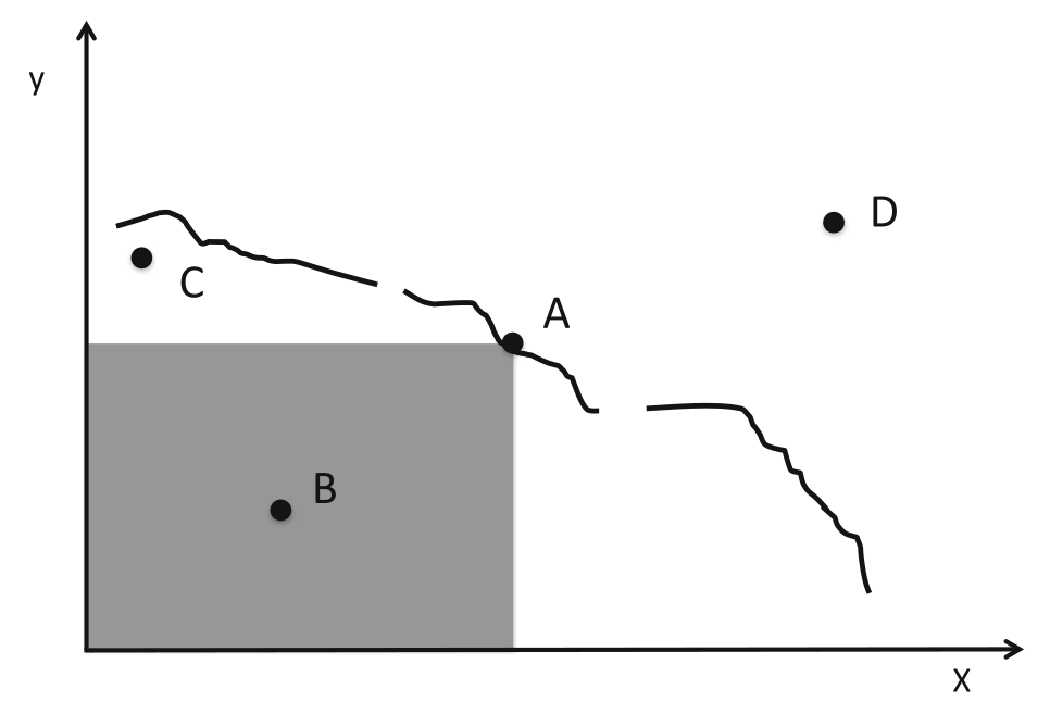
The x- and y-axes represent two conflicting objectives subject to
constraints.
The quality of solutions is represented by their x and y values (larger
is better).
Point A dominates B and all other points in the grey area.
A and C do not dominate each other.
The line represents the Pareto set, of which point A is an
example.
Solutions above and to the right of the line, such as D, are
infeasible
In the figure, this front is illustrated for two conflicting
objectives,
that are both to be maximised.
This figure also illustrates some of the features,
such as non-convexity and discontinuities,
frequently observed in real applications,
that can cause particular problems for traditional optimisation
techniques,
using often sophisticated variants of scalarisation to identify the
Pareto set.
EAs have a proven ability to identify high-quality solutions,
in high-dimensional search spaces containing difficult features,
such as discontinuities and multiple constraints.
When coupled with their population-based nature,
and their ability for finding and preserving diverse sets of good
solutions,
it is not surprising that EA-based methods are currently the state of
the art,
in many multiobjective optimisation problems.
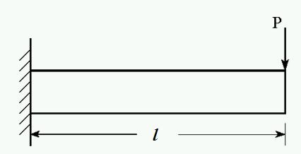
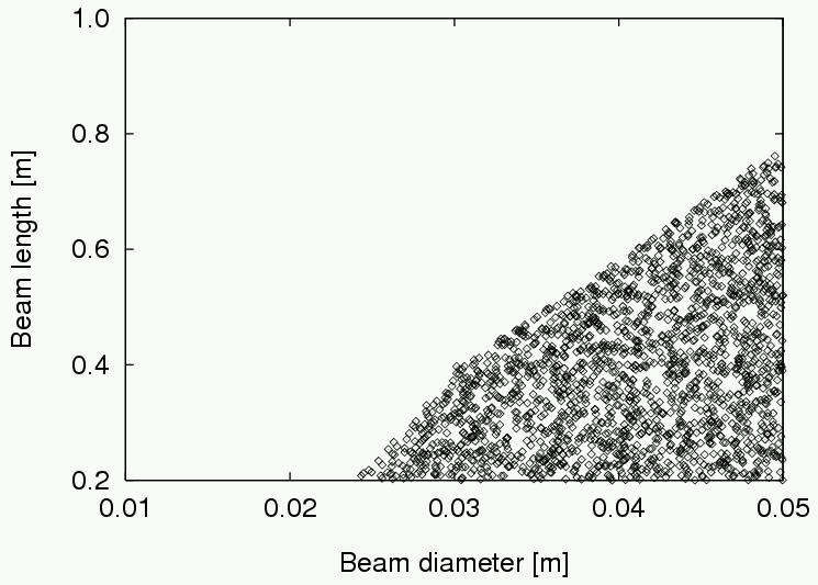
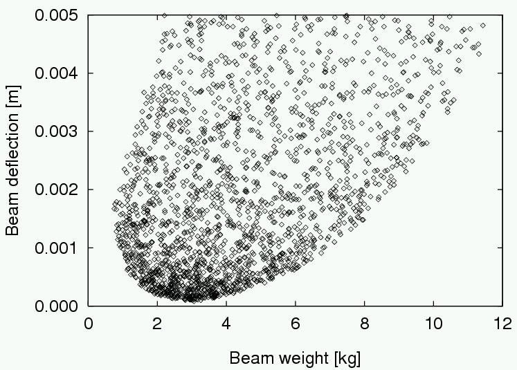
A practical example is the following beam design problem.
Minimize weight and deflection of a beam (Deb, 2001):
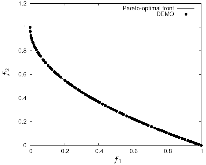
Goal: Finding non-dominated solutions

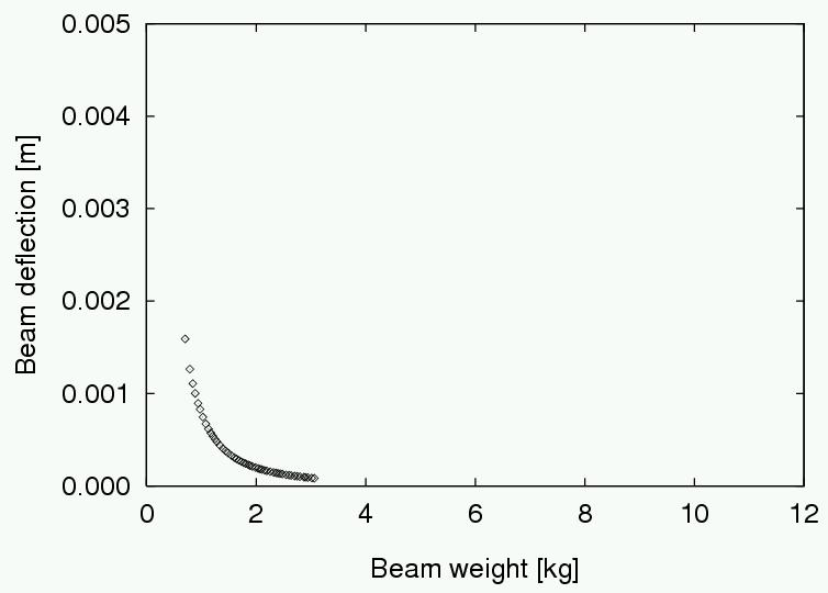
Find a set of non-dominated solutions (approximation set) following
the criteria of:
convergence (as close as possible to the Pareto-optimal front),
diversity (spread, distribution).
| Characteristic | Singleobjective optimisation | Multiobjective optimisation |
|---|---|---|
| Number of objectives | one | more than one |
| Spaces | single | two: decision (variable) space, objective space |
| Comparison of candidate solutions | x is better than y | x dominates y |
| Result | one (or several equally good) solution(s) | Pareto-optimal set |
| Algorithm goals | convergence | convergence, diversity |
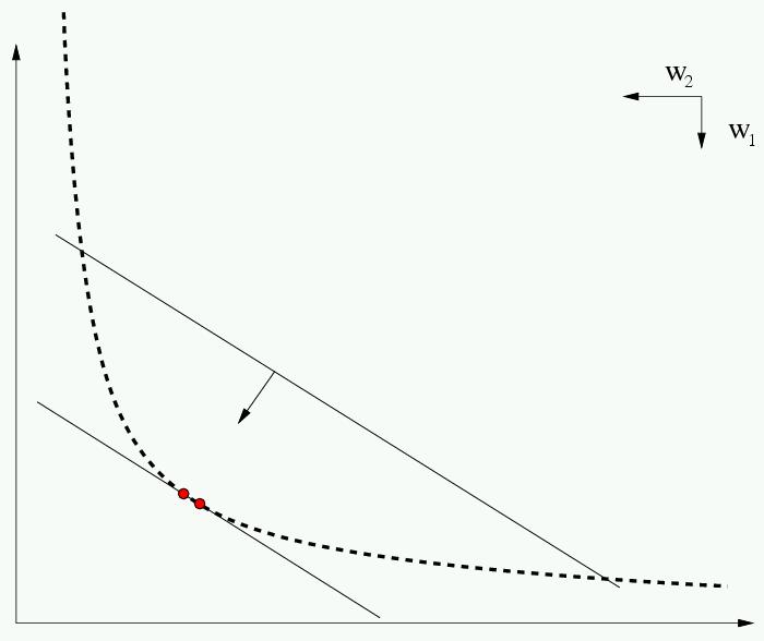
Traditional, using single (aggregated) objective optimization methods.
An example approach: Weighted-sum
H yperplanes in the objective space!
Ideally, we don’t aggregate fitnesses:
Possible with novel multiobjective optimization techniques,
enabling better insight into the problem.
Given a multiobjective optimization problem,
use higher-level information on importance of objectives,
to transform the problem into a single objective one,
and then solve it with a single objective optimization method
to obtain a particular trade-off solution.
Given a multiobjective optimization problem,
solve it with a multiobjective optimization method
to find multiple trade-off solutions,
and then use higher-level information
to obtain a particular trade-off solution.
There have been many approaches to multiobjective optimisation using
EAs,
beginning with Schaffer’s vector-evaluated genetic algorithm (VEGA) in
1984.
In this algorithm the population was randomly divided into
subpopulations,
that were then each assigned a fitness (and subject to selection),
according to a different objective function,
but parent selection and recombination were performed globally.
This modification preserved an approximation to the Pareto front,
for a few generations, but not indefinitely.
Goldberg suggested the use of fitness based on dominance,
rather than on absolute objective scores,
coupled with niching and/or speciation methods to preserve
diversity,
and this breakthrough triggered a dramatic increase in research activity
in this area.
We briefly describe some of the best-known algorithms below,
noting that the choice of representation, and hence variation
operators,
are entirely problem dependent,
and so we concentrate on the way that fitness assignment and selection
are performed.
Some algorithms explicitly exert selection pressure towards the discovery of nondominated solutions.
Fonseca and Fleming’s multiobjective genetic algorithm (MOGA):
assigns a raw fitness to each solution,
equal to the number of members of the current population that it
dominates, plus one.
It uses fitness sharing amongst solutions of the same rank,
coupled with fitness-proportionate selection to help promote
diversity.
Srinivas and Deb’s nondominated sorting genetic algorithm
(NSGA):
works in a similar way, but assigns fitness based on dividing the
population,
into a number of fronts of equal domination.
The algorithm iteratively seeks all the nondominated points in the
population,
that have not been labelled as belonging to a previous front.
It then labels the new set as belonging to the current front,
and increments the front count,
repeating until all solutions have been labelled.
Each point in a given front gets as its raw fitness,
the count of all solutions in inferior fronts.
Again fitness sharing is implemented to promote diversity,
but this time it is calculated considering only members from that
individual’s front.
Horn et al.’s niched Pareto genetic algorithm (NPGA):
differs in that it uses a modified version of tournament
selection,
rather than fitness proportionate with sharing.
The tournament operator works by comparing two solutions,
first on the basis of whether they dominate each other,
and then second on the number of similar solutions already in the new
population.
Although all three of these algorithms show good performance on a number
of test problems,
they share two common features:
1. performance depends on a suitable choice of parameters in the
sharing/niching procedures.
2. they can potentially lose good solutions.
During the 1990s much work was done elsewhere in the EA research
community,
developing methods for reducing dependence on parameter settings.
Theoretical breakthroughs were achieved,
showing that single-objective EAs converge to the global optimum on some
problems,
providing that an elitist strategy was used.
In the light of this research, Deb and coworkers proposed the revised
NSGA-II,
which still uses the idea of non-dominated fronts, but incorporates the
following changes:
A crowding distance metric is defined, for each point,
as the average side length of the cuboid,
defined by its nearest neighbours in the same front.
The larger this value, the fewer solutions reside in the vicinity of the
point.
A \((\mu + \lambda)\) survivor selection strategy is used (with \(\mu = \lambda\)).
The two populations are merged and fronts assigned.
The new population is obtained by accepting individuals,
from progressively inferior fronts, until it is full.
If not all of the individuals in the last front considered can be
accepted,
then they are chosen on the basis of their crowding distance.
Parent selection uses a modified tournament operator,
that considers first dominance rank then crowding distance.
As can be seen, this achieves elitism (via the plus strategy),
and an explicit diversity maintenance scheme,
as well as reduced dependence on parameters.
Two other prominent algorithms,
the strength Pareto evolutionary algorithm (SPEA-2), and
the Pareto archived evolutionary strategy (PAES),
both achieve the elitist effect, in a slightly different way by,
using an archive containing a fixed number of nondominated points,
discovered during the search process.
Both maintain a fixed sized archive,
and consider the number of archived points close to a new
solution,
as well as dominance information, when updating the archive.
How can we maintain diversity of solutions?
It should be clear from the descriptions of the MOEAs above,
that all of them use explicit methods to enforce preservation of
diversity,
rather than relying simply on implicit measures,
such as parallelism (in one form or another) or artificial
speciation.
In single-objective optimisation,
explicit diversity maintenance methods are often combined with implicit
speciation methods,
to permit the search for optimal solutions, within the preserved
niches.
The outcome of this, is a few highly fit diverse solutions,
often with multiple copies of each.
In contrast to this, the aim of MOEAs is to attempt to distribute the
population evenly,
along the current approximation to the Pareto front.
This partially explains why speciation techniques have not been used in
conjunction with the explicit measures.
Finally, it is worth noting that the more modern algorithms discussed,
have abandoned fitness sharing,
in favour of direct measures of the distance to the nearest
non-dominating solution, more akin to crowding.
An un-avoidable problem of trying to evenly represent an
approximation of the Pareto front,
is that this approach does not scale well,
as the dimensionality of the solution space increases above 5–10
objectives.
One recent method that has gathered a lot of attention,
is the decomposition approach taken by Zhang’s MOEA-D algorithm,
which shares features from both:
the single-objective weighted sum approach and
the population-based approaches.
Rather than use a single weighted combination,
MOEA-D starts by evenly distributing a set of N weight vectors in the
objective space,
and for each building a list of its T closest neighbours
(measured by Euclidean distances between them).
It then creates and evolves a population of N individuals,
each associated with one of the weight vectors,
and uses it to calculate a single fitness value.
What differentiates this from simply being N parallel independent
searches,
is the use of the neighbourhood sets to structure the population,
with selection and recombination only happening within demes, as in
cellular EAs.
Periodically, the location of the weight vectors and the neighbour sets
are recalculated,
so that the focus of the N parallel searches reflects what has been
discovered about the solution space.
MOEA-D, and variants on the original algorithm,
have been shown to perform equivalently to dominance-based methods in
low dimensions,
and to scale far better to many-objective problems with 5 or more
conflicting dimensions.
Distributed Coevolution of Job Shop Schedules
An interesting application can be seen:
Husbands’ distributed coevolutionary approach to multiobjective
problems.
He uses a coevolutionary model to tackle a complex multiobjective,
multi-constraint problem,
namely a generalised version of job shop scheduling.
Here a number of items need to be manufactured,
each requiring a number of operations on different machines.
Each item may need a different number of operations,
and in general the order of the operations may be varied,
so that the problem of finding an optimal production plan for one item
is itself NP-hard.
The usual approach to the multiple task problem is to optimise each plan
individually,
and then use a heuristic scheduler to interleave the plans so as to
obtain an overall schedule.
However, this approach is inherently flawed,
because it optimises the plans in isolation,
rather than taking into consideration the availability of machines,
etc.
Husbands’ approach is different:
He uses a separate population to evolve plans for each item and
optimises these concurrently.
In this sense we have a MOP,
although the desired final output is a single set of plans (one for each
item),
rather than a set of diverse schedules.
A candidate plan for one item gets evaluated in the context of a member
from each other population,
i.e., the fitness value (related to time and machining costs) is for a
complete production schedule.
An additional population is used to evolve ‘arbitrators’,
which resolve conflicts during the production of the complete
schedule.
Early experiments experienced problems with premature loss of
diversity.
These problems are treated by the use of an implicit approach to
diversity preservation,
namely the use of a diffusion model EA.
Furthermore, by colocating one individual from each population in each
grid location,
the problem of partner selection is neatly solved:
a complete solution for evaluation corresponds to a grid cell.
We will not give details of Husbands’ representation and variation
operators here,
as these are highly problem specific.
Rather we will focus on the details of his algorithm,
that were aimed at aiding the search for high-class solutions.
The first of these is, of course, the use of a coevolutionary
approach.
If a single population were used,
with a solution representing the plans for all items,
then there would be a greater likelihood of genetic hitchhiking,
whereby a good plan for one item in the initial population would take
over,
even if the plans for the other items were poor.
By contrast, the decomposition into different subpopulations,
means that the good plan can at worst take over one population.
The second feature that aids the search over diverse local optima
is:
the use of a diffusion model approach.
The implementation uses a 15-by-15 square toroidal grid, thus a
population size of 225.
Plans for 5 items, each needing between 20 and 60 operations, were
evolved,
so in total there were 6 populations,
and each cell contained a plan for each of the 5 items plus an
arbitrator.
A generational approach is used:
Within each generation each cell’s populations are ‘bred’,
with a random permutation to decide the order in which cells are
considered.
The breeding process within each cell is iterated for each population
and consists of the following steps:
Generate a set of points to act as neighbours,
by iteratively generating random lateral and vertical offsets from the
current position.
A binomial approximation to a Gaussian distribution is used,
which falls off sharply for distances more than 2 and is truncated to
distance 4.
Rank the cells in this neighbouhood according to cost,
and select one using linear ranking with s = 2.
Take the member of the current population from the selected
cell,
and the member in the current cell,
and generate an offspring via recombination and mutation.
Choose a cell from the neighbourhood using inverse linear ranking.
Replace the member of the current population in that cell with the newly created offspring.
Re-evaluate all the individuals in that cell using the newly
created offspring.
The results presented from this technique showed that the system
managed
to evolve low-cost plans for each item, together with a low total
schedule time.
Notably, even after several thousand iterations, the system had still
preserved
a number of diverse solutions.
Population-based method.
Can return a set of trade-off solutions (approximation set) in a single
run.
Allows for the ideal approach to multiobjective optimization.
Population-based nature of search means you can
simultaneously search,
for the set of points approximating Pareto front.
You don’t have to make guesses about which combinations of weights might
be useful.
It makes no assumptions about shape of Pareto front, which can be convex
/ discontinuous etc.
MO problems occur very frequently
EAs are very good in solving MO problems
MOEAs are one of the most successful EC subareas
Lexicase + Novelty search for phenotypic and genotypic diversity from
the entire past population
Reward any solution that does best on objective function, or one that is
most novel.