Epidemiology is a formal branch of science focusing
on the study of space-time patterns of illness in a population and the
factors that contribute to these patterns.
Computational epidemiology is an interdisciplinary
area setting its sights on developing and using computer models to
understand and control the spatiotemporal diffusion of disease through
populations.
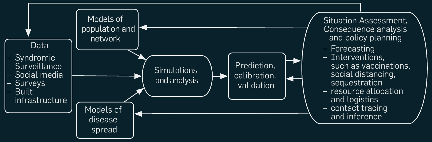
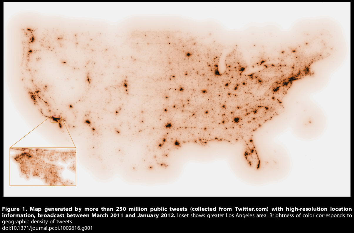
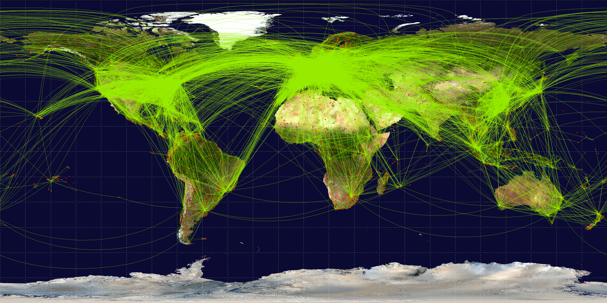
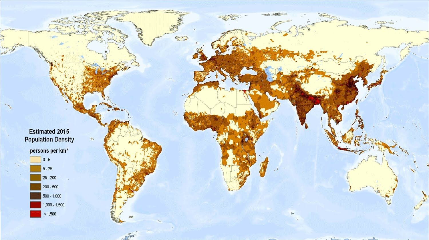
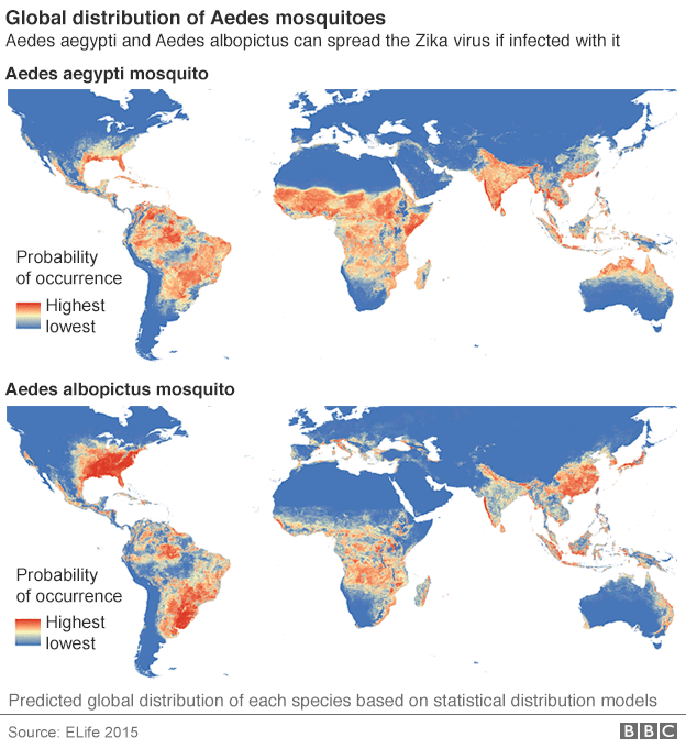
* The process starts by developing models of synthetic social contact
networks and within host disease progression using diverse datasets that
include: surveys, census, social media, serological investigations, and
disease surveillance.
* High-performance computer simulations are then used to study the
dynamics of disease propagation and the effects of various intervention
strategies.
* The results are used by policymakers and analysts to formulate and
evaluate various public policies as well as putative societal
responses.
* All these models are refined, based on the simulation results and the
policies being studied.
1.3 Historical
1.3.1 SIR model
24-CompEpi/sir_pop.png
1.3.1.1 SIR over time
24-CompEpi/sir3.png
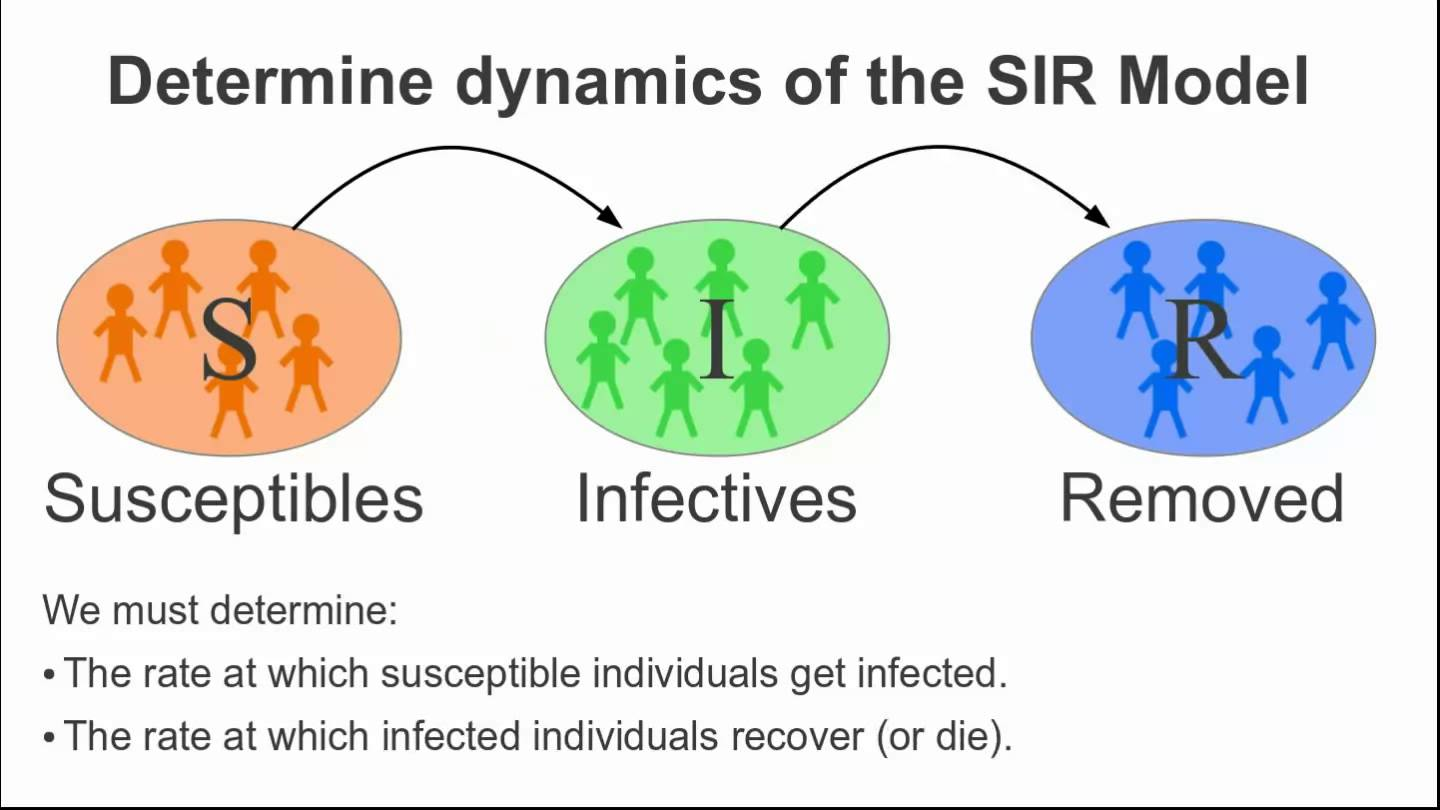
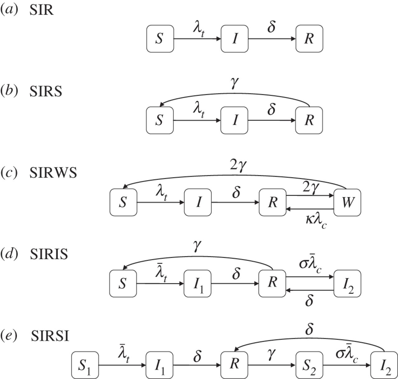
* The simplest aggregate model is popularly known as the SIR
model.
* A population of size N is divided into three states: susceptible (S),
infective (I), and removed or recovered (R).
* The following discrete time process describes the system
dynamics:
* each infected person can infect any susceptible person (independently)
with probability \(\beta\), and can
recover with probability \(\gamma\).
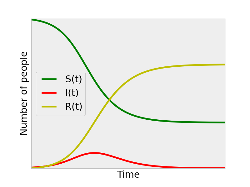
* Let S(t), I(t) and R(t) denote the number of people who are
susceptible, infected and recovered states at time t,
respectively.
* Let: \(s(t) = S(t)/N \\ i(t) = I(t)/N \\ r(t) =
R(t)/N\)
then, \(s(t) + i(t) + r(t) = 1\)
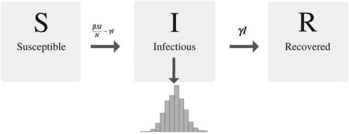
By the “complete mixing” assumption that each individual is in contact
with everyone in the population, it can be shown that the following
system of differential equations (known as the SIR model) describes the
dynamics: \(\frac{ds(t)}{dt} = - \beta s(t) i(t) \\
\frac{di(t)}{dt} = \beta s(t) i(t) - \gamma i(t)\\ \frac{dr(t)}{dt} =
\gamma i(t)\)
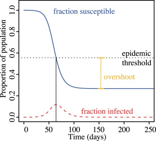
* One of the classic results in the SIR model is there is an epidemic
that infects a large fraction of the population, if and only if \(R_0 = \beta / \gamma > 1\);
* The parameter \(R_0\) is known as the
“reproductive number,” and thus much of public health decision making is
centered on controlling \(R_0\).
1.3.1.2 Similar models
24-CompEpi/sir.png
1.3.1.3 Threshold
24-CompEpi/sir4.png
1.4 Modern
1.4.1 Networked epidemiology
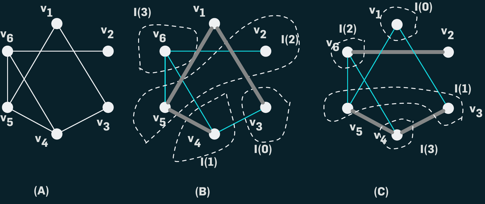
a. Example showing a contact network on a population of size 6,
represented by the set of nodes {v1, v2, v3, v4, v5, v6}.
b. An example of a dendogram on this contact graph, with the infected
sets I(t), t = 0, 1, 2, 3 as shown.
* The teal edges represent the edges on which the infections
spread.
* The infection starts at node v3, and eventually all nodes, except v1
get infected; the epicurve corresponding to this example is (1, 1, 2,
1), with the peak being at time 2.
c. Another possible dendogram on the same network, with the infection
starting at v1, where all nodes except v2 get infected.
1.4.2 Process of generating a
networked model
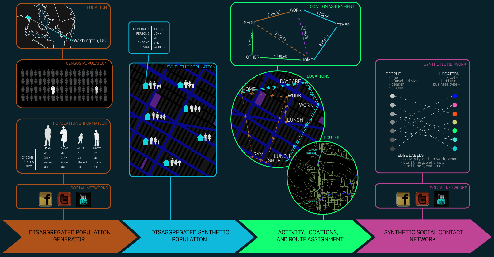
* Step 1. Construct a synthetic yet realistic population by integrating
a variety of commercial and public sources.
* Step 2. Build a set of detailed activity templates for households
using time-use surveys and digital traces. Assigns daily activities to
individuals within a household using activity and time-use surveys as
well as information available from social media.
* Step 3. Construct a dynamic social bipartite visitation network, GPL,
which encodes the locations visited by each person. Constructs a dynamic
social bipartite visitation network, represented by a (vertex and edge)
labeled bipartite graph GPL, where P is the set of people and L is the
set of locations.
* Step 4. Develop models of within-host disease progression using
detailed case-based data and serological samples to establish disease
parameters.
* Step 5. Develop high-performance computer simulations to study
epidemic dynamics (exploring the Markov chain M).
* Step 6. Develop multi-theory multi-network models of individual,
collective, and organizational behaviors, formulating and evaluating the
efficacy of various intervention strategies and methods for situation
assessment and epidemic forecasting.
1.4.2.1 Step 1
Step 1:
* Construct a synthetic population statistically similar to census, by
integrating a variety of commercial and public sources.
* We create synthetic urban populations by integrating a variety of
databases from commercial and public sources into a common architecture
for data exchange that preserves the confidentiality of the original
data sets, and yet produces realistic attributes and demographics for
the synthetic individuals.
* A census of our synthetic population yields results that are
statistically indistinguishable from the original census data, if they
are both aggregated to the block group level; this is illustrated in the
schematic.
1.4.2.2 Step 2
Step 2:
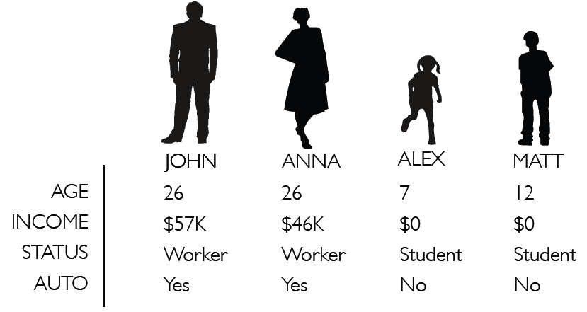
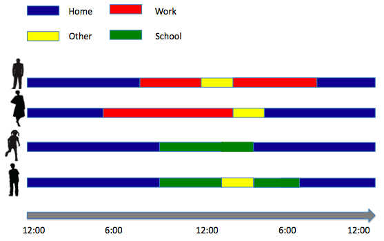
* Build a set of detailed activity templates for households based on
activity and time-use surveys A set of activity templates for
individuals in the households are determined, based on US census and
survey data on activity and time-use surveys.
* These activity templates describe the sort of activities each
household member performs and the time of day they are performed; a
sample of such activity templates is shown.
1.4.2.3 Step 3
Step 3:
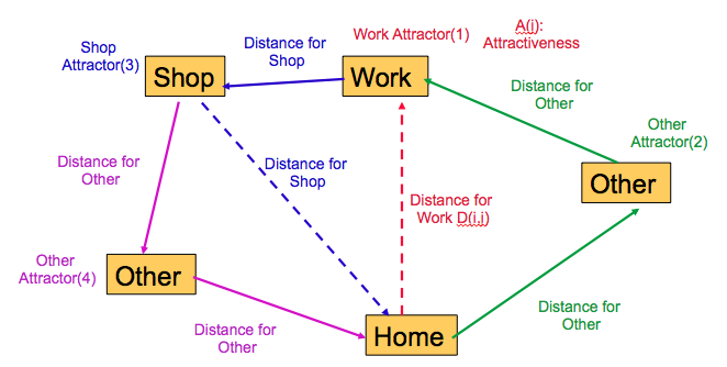
* Construct a dynamic social bipartite visitation network, GPL, which
encodes the locations visited by each person.
* The next step involves selecting locations where each of these
activities are performed, for every person.
* Detailed statistical models developed in the transportation literature
are used for this step; these are typically gravity models, which
involve selecting locations based on a power of the distance.
* This is illustrated in the figure.
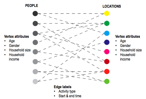
* The movement of people from one location to the next in their activity
sequence is done by routing on the transportation network.
* By using a cellular automaton model for the actual movement, we get a
very detailed spatio-temporal model of people.
* For the purpose of this paper, we use a bipartite graph representation
of the this mobility, involving people and locations, as shown in the
figure below.
1.4.2.4 Step 5
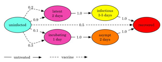
* Models of disease progression are represented as probabilistic timed
transition systems or PTTS, as shown in the figure.
* These are finite state systems with two additional features:
transitions are triggered sometimes as a timed event and they can be
probabilistic.
* In the example PTTS for a strain of flu in the figure below, an
individual can transition to a latent state with probability 0.9 or to
an incubating state with probability 0.1, if untreated; these
probabilities change if the individual is vaccinated.
* If the person reaches a latent state, he switches to an infectious
state in 2 days, during which time he can spread the infection to his
uninfected and susceptible neighbors with some probability.
* Finally he switches to a recovered state in 3-5 days.
* The simulation of epidemic models on large populations involves
evaluation over a network with a PTTS for every node.
* This is computationally very challenging, and we have developed four
different simulation tools, that are relevant for different kinds of
problems: EpiSims, EpiSimdemics, EpiFast and Indemics.
* Their performance is summarized in the table below.
1.4.3 Extensions of the basic
model
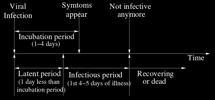
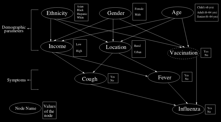
1.4.3.1 Timeline and Bayesian
24-CompEpi/timeline.png24-CompEpi/bayes.png
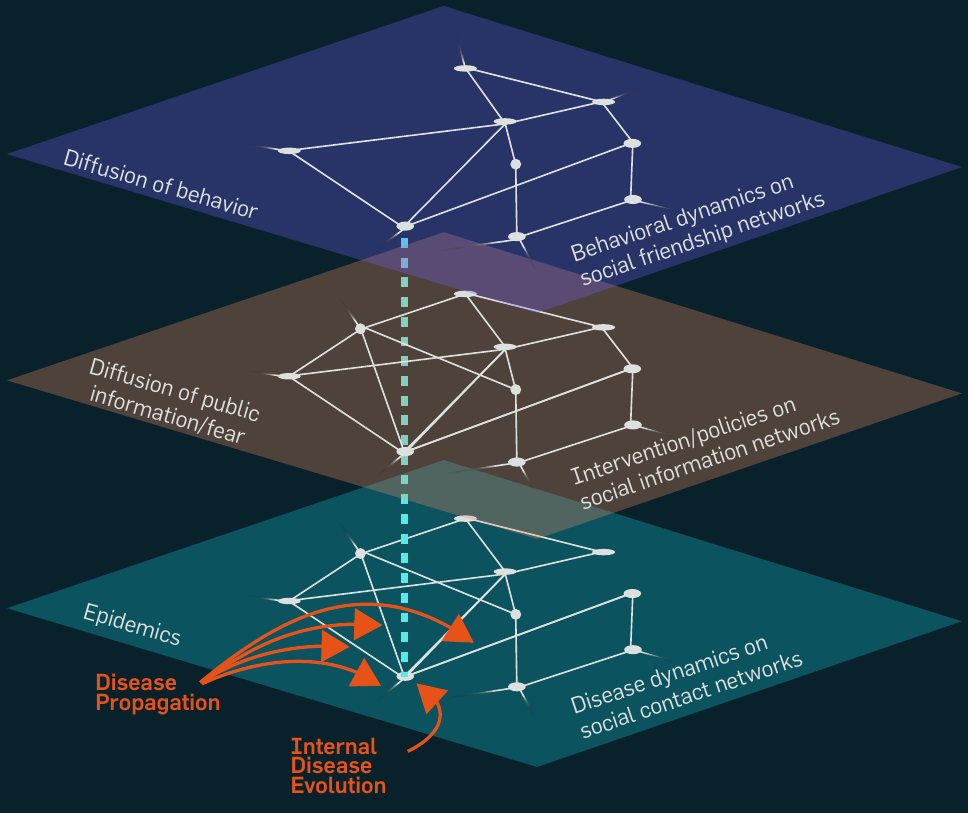
1.4.3.2 Other layers
* The layers represent examples of different kinds of networks in which
the nodes might be involved.
* The bottom layer is a social contact network formed by co-location
constraints, on which diseases spread.
* The middle layer is an information network, on which information/fear
spread.
* Finally, the top layer is a friendship network that spreads influence,
for example, peer pressure.