Previous: 22-BioNetworks.html
Layout is just the display, and
there can be many layouts for one actual graph.
Even when nodes have a position in physical space,
the position of the nodes in a layout,
often has no relation to their position in actual space.
https://en.wikipedia.org/wiki/Network_theory
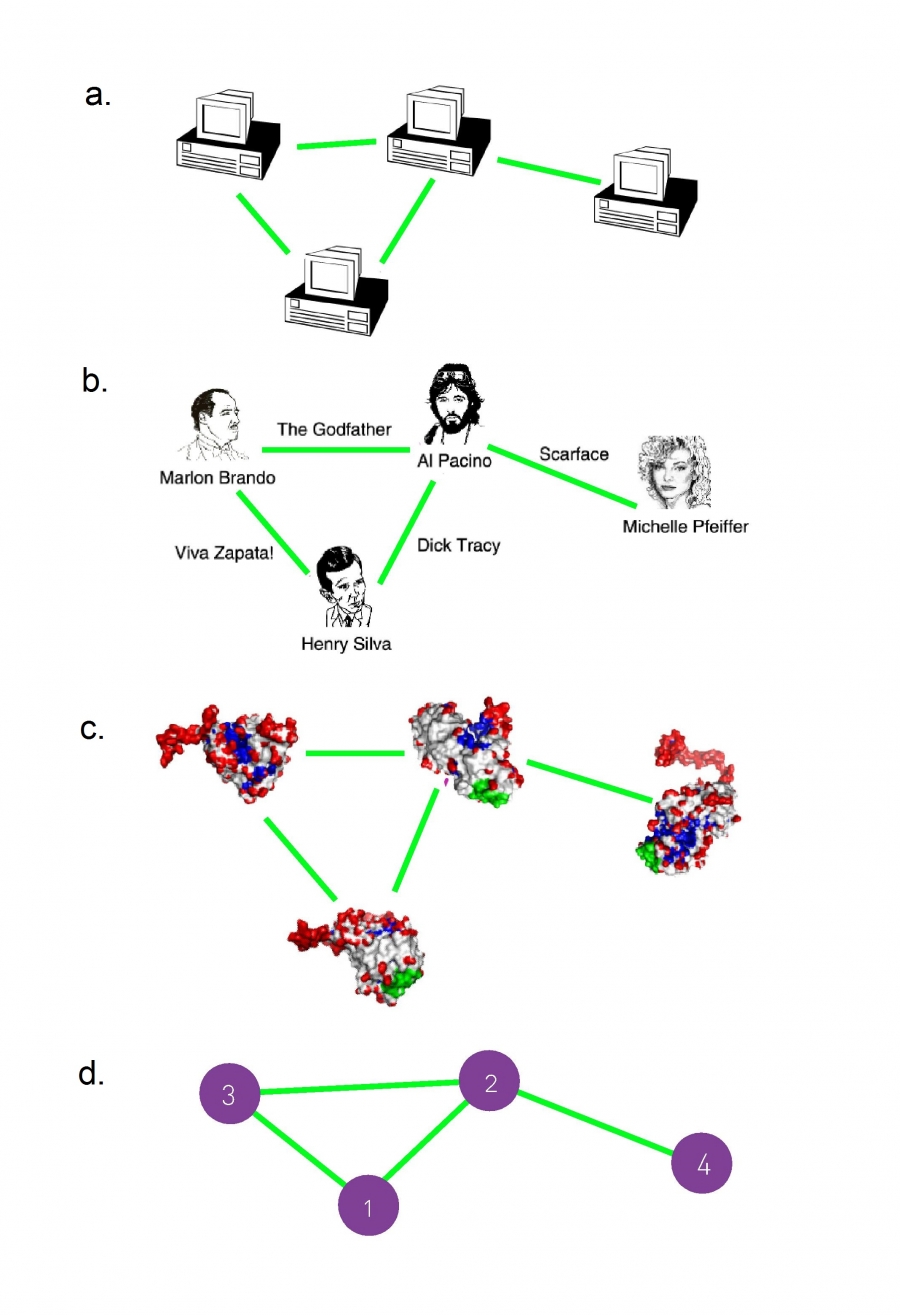
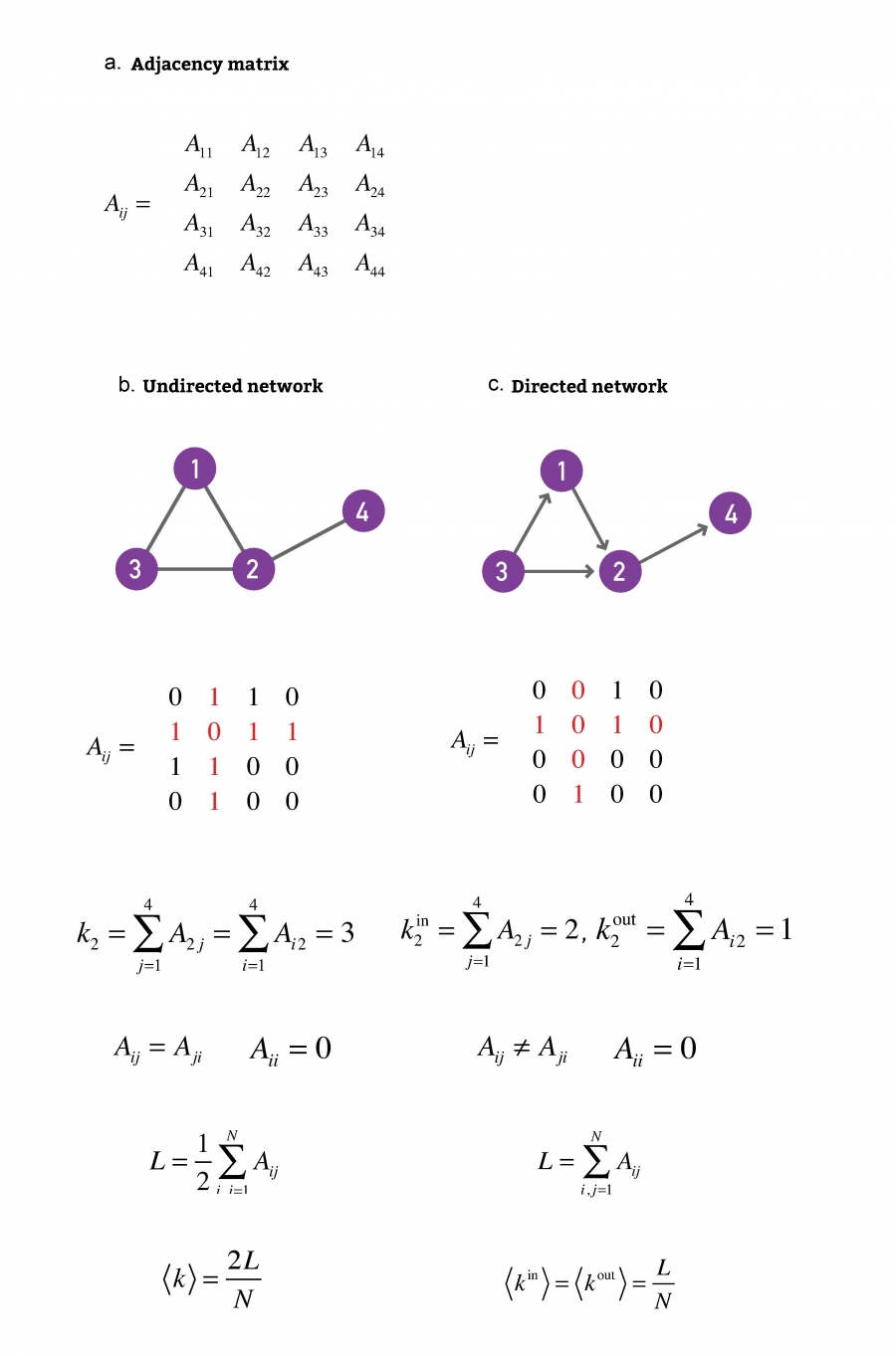
Number of nodes, or N,
represents the number of components in the system.
We will often call N the size of the network.
To distinguish the nodes,
we label them with i = 1, 2, …, N.
Number of links, which we denote with
L,
represents the total number of interactions between the nodes.
Links are rarely labeled,
as they can be identified through the nodes they connect.
For example, the (2, 4) link connects nodes 2 and 4.
The networks shown here have N = 4 and L = 4.
https://en.wikipedia.org/wiki/Degree_(graph_theory)
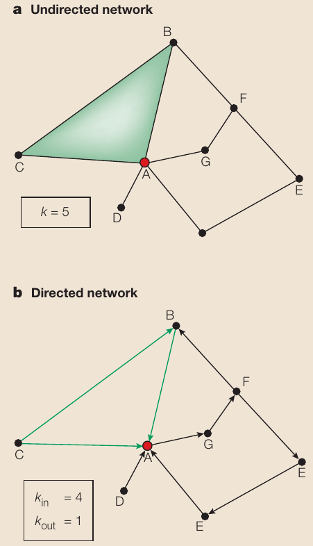
One elementary characteristic of a node is its degree (or connectivity),
k,
which tells us how many links the node has to other nodes.
For each node i,
we can describe its degree (k) with ki,
the number of connections of the ith node in the
network,
The sum of all ki relates to L,
the number of links of the whole network.
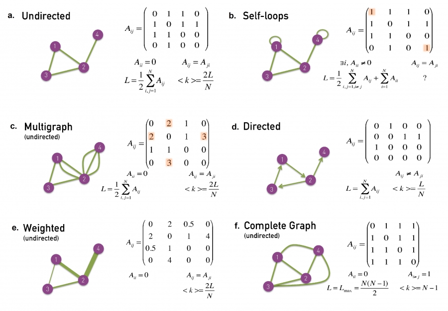
In an undirected network
The total number of links can be described in terms of the sum of all
node’s degrees:
\(L = \frac{1}{2}\sum\limits_{i = 1}^N {k_i
}\)
The average degree of a node is:
\(\left\langle k \right\rangle =
\frac{1}{N}\sum\limits_{i = 1}^N {k_i } = \frac{{2L}}{N}\)
In an directed network
The number of links:
\(L = \sum\limits_{i = 1}^N {k_i^{in} } =
\sum\limits_{i = 1}^N {k_i^{out} }\)
The average degree
\(\left\langle {k^{in} } \right\rangle =
\frac{1}{N}\sum\limits_{i = 1}^N {k_i^{in} } = \left\langle {k^{out} }
\right\rangle = \frac{1}{N}\sum\limits_{i = 1}^N {k_i^{out} } =
\frac{L}{N}\)
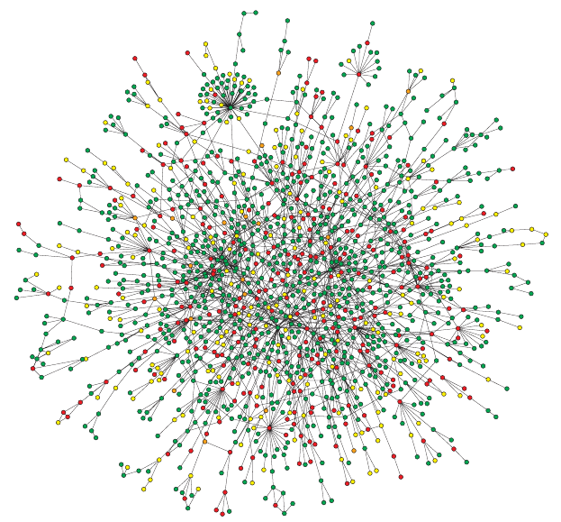
Below: Yeast protein interaction network.
A map of protein-protein interactions in Saccharomyces cerevisiae,
which is based on early yeast two-hybrid measurements,
illustrates that a few highly connected nodes
(which are also known as hubs) hold the network together.
The largest cluster, which contains ~78% of all proteins, is
shown.
The color of a node indicates a phenotypic effect,
of removing the corresponding protein:
(red = lethal, green = non-lethal, orange = slow growth, yellow =
unknown).
How do we know that?
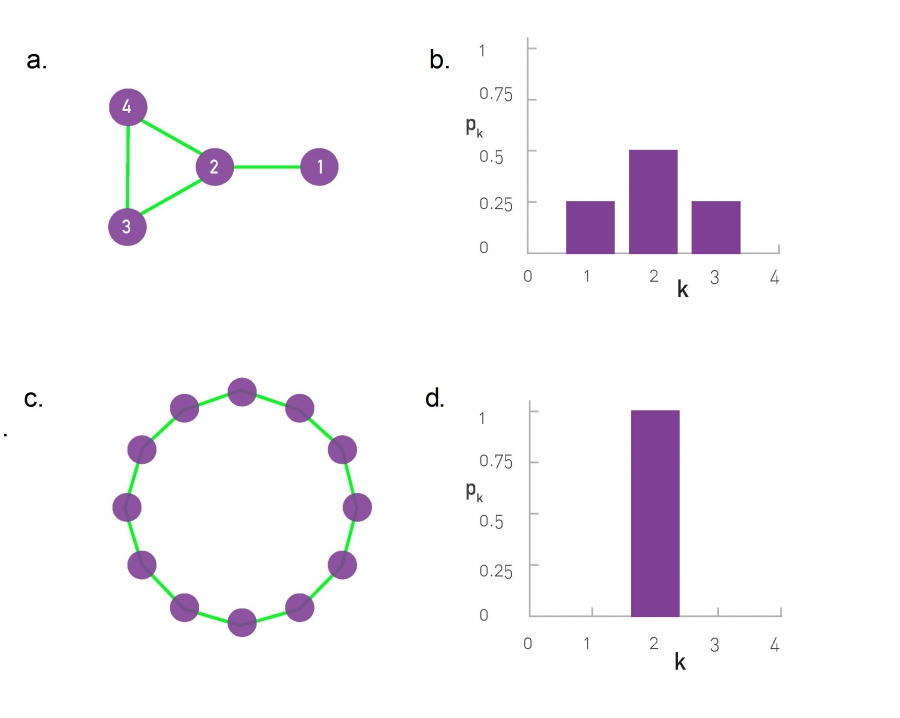
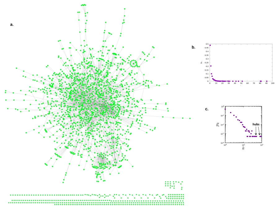
Degree Distribution of a Gene Network
In real-world networks the node degrees can vary widely.
Below, is a layout of the protein interaction network of yeast.
Each node corresponds to a yeast protein, and
links correspond to experimentally detected binding interactions.
The proteins shown on the bottom have self-loops, hence for them
k=2.
The degree distribution of the protein interaction network shown in
(a).
The observed degrees vary between k=0 (isolated nodes) and k=92,
which is the degree of the most connected node, called a hub.
There are also wide differences in the number of nodes with different
degrees:
Almost half of the nodes have degree one
(i.e. p1=0.48),
while we have only one instance of the biggest k (i.e. p92 =
1/N=0.0005).
The degree distribution is often shown on a log-log plot,
in which we either:
plot log pk in function of ln(k), or
we use logarithmic axes.
The degree distribution P(k) of a network is then defined to be:
the fraction of nodes in the network with degree k.
Thus if there are n nodes in total in a network,
and nk of them have degree k, then we have:
\(P(k)={\frac {nk}{n}}\)
X-axis is the k itself,
Y-axis is like a count (a proportion).
Human brain degree predicts regional involvement with disease
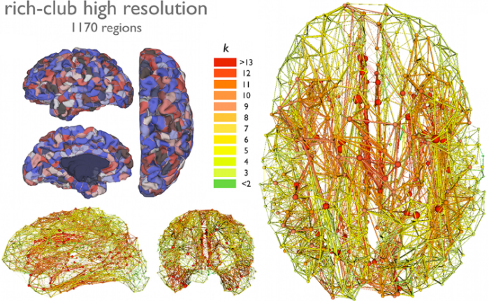
The regions with higher degree are more likely to be involved in
neurodegeneration.
Adjacency matrix
Adjacency list
Edge list
https://en.wikipedia.org/wiki/Adjacency_matrix
What is an adjacency matrix?
A matrix whose rows and columns are indexed by vertices,
and whose cells contain a Boolean value,
indicating whether an edge is present between the vertices,
corresponding to the row and column of the cell.
https://en.wikipedia.org/wiki/Adjacency_list
An adjacency list is a collection of unordered lists.
Each unordered list within an adjacency list describes:
the set of neighbors of a particular vertex in the graph.
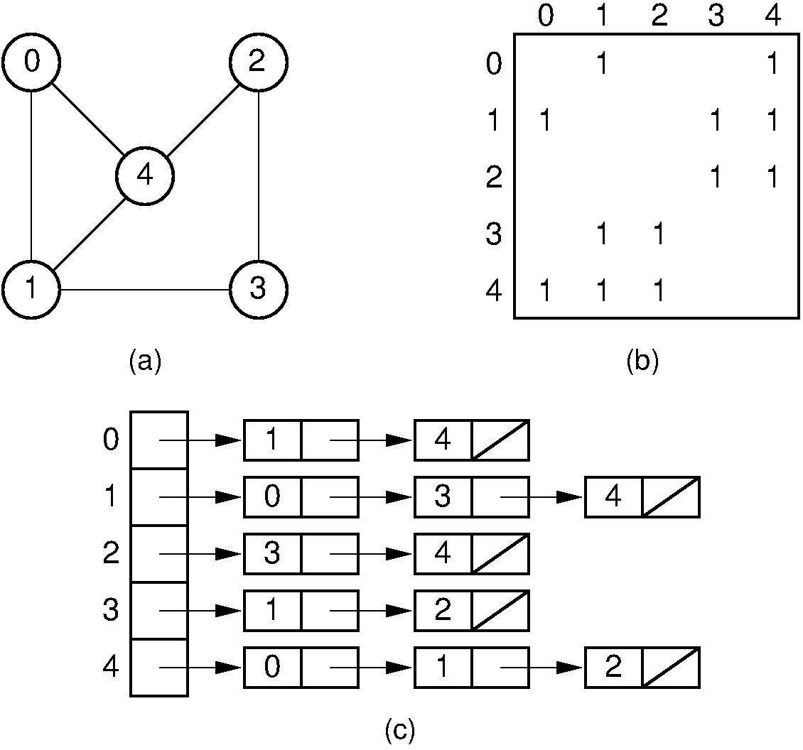
a) graph,
b) matrix,
c) list
For a sparse graph,
one in which most pairs of vertices are not connected by edges,
an adjacency list is significantly more space-efficient,
compared to an adjacency matrix (stored as an array).
The space usage of the adjacency list,
is proportional to the number of edges and vertices in the graph,
while for an adjacency matrix stored in this way,
the space is proportional to the square of the number of vertices.
It is possible to store adjacency matrices more space-efficiently,
matching the linear space usage of an adjacency list,
by using a hash table indexed by pairs of vertices,
rather than an array.
Another significant difference between adjacency lists and adjacency
matrices,
is in the efficiency of the operations they perform:
In an adjacency list,
the neighbors of each vertex may be listed efficiently,
in time proportional to the degree of the vertex.
In an adjacency matrix,
this operation takes time proportional to the number of vertices in the
graph,
which may be significantly higher than the degree.
The adjacency matrix allows testing whether:
two vertices are adjacent to each other in constant time.
The adjacency list is slower to support this operation.
Max L on undirected simple graph:
\(L_{\max } = \frac{{N(N -
1)}}{2}\)
Why?
This graph was constructed under constraint by simple rules:
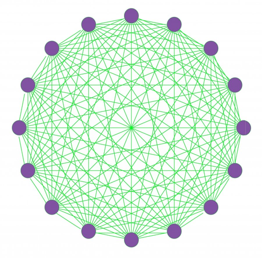 t
t
This is not a realistic network.
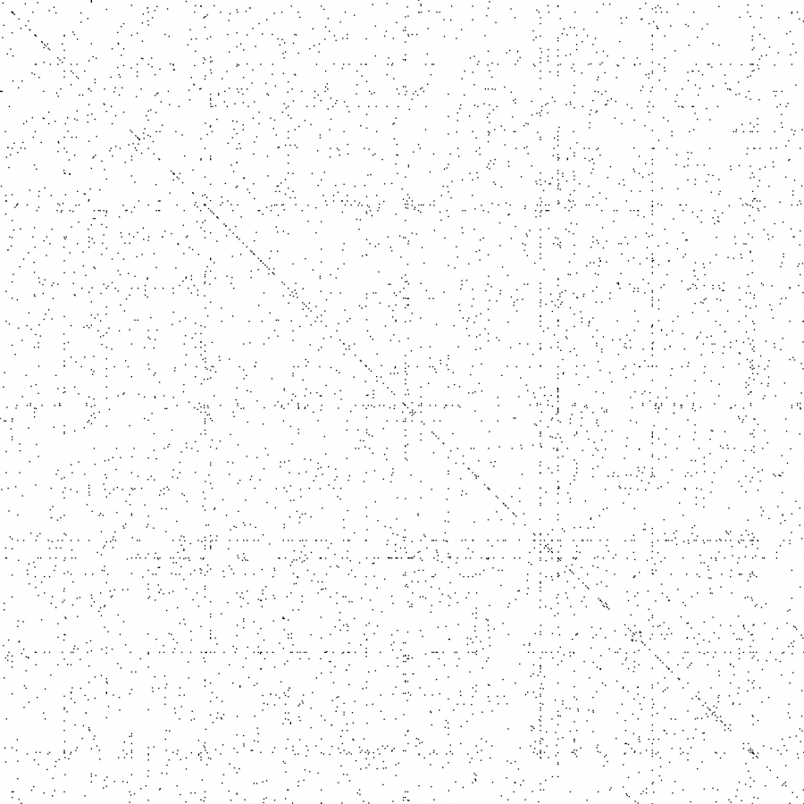
Below, we see:
a sparse adjacency matrix,
representing the yeast protein-protein interaction network,
consisting of 2,018 nodes,
each representing a yeast protein.
For each position of the adjacent matrix where:
Aij = 1, A dot is placed
indicating the presence of an interaction.
There are no dots for Aij = 0.
The small fraction of dots illustrates what?
The sparse nature of the real protein-protein interaction network.
https://en.wikipedia.org/wiki/Bipartite_graph
How do we model the interaction between two separate sets of
nodes,
when nodes themselves in each may be related only to the other
set,
but not to each other directly?
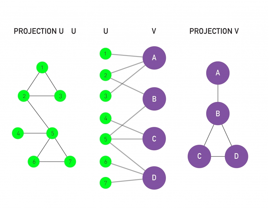
A bipartite network has two sets of nodes, U and V.
Nodes in the U-set connect directly only to nodes in the V-set.
Hence there are no direct U-U or V-V links.
A bipartite graph (or bigraph) is a network,
whose nodes can be divided into two disjoint sets U and V,
such that each link connects a U-node to a V-node.
If we color the U-nodes green and the V-nodes purple,
then each link must connect nodes of different colors.
We can generate two projections for each bipartite network:
The first projection connects two U-nodes by a link,
if they are linked to the same V-node in the bipartite
representation.
The second projection connects the V-nodes by a link,
if they connect to the same U-node.
The figure shows the two projections we can generate from any bipartite network.
Projection U is obtained by:
connecting two U-nodes to each other,
if they link to the same V-node in the bipartite representation.
Projection V is obtained by:
connecting two V-nodes to each other,
if they link to the same U-node in the bipartite network.
Medicine offers another prominent example of a bipartite
network:
The Human Disease Network connects diseases to genes,
whose mutations are known to cause or effect the corresponding
disease.
One projection of the diseaseome is the disease network,
whose nodes are diseases.
Two diseases are connected,
if the same genes are associated with them,
indicating that the two diseases have common genetic origin.
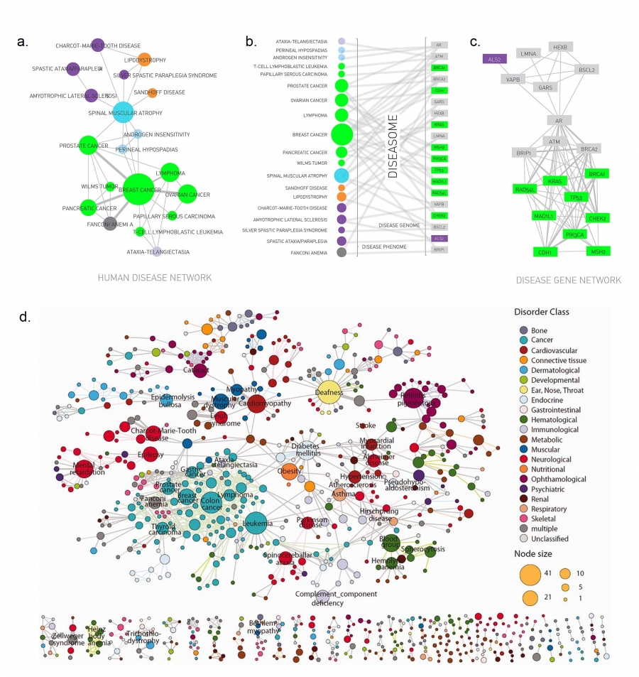
(a)-(c) shows a subset of the diseaseome,
focusing on cancers.
The Human Disease Network (or diseaseome) is a bipartite network,
whose nodes are diseases (U) and genes (V).
A disease is connected to a gene,
if mutations in that gene are known to affect the particular
disease.
The second projection is the gene network,
whose nodes are genes, and
where two genes are connected,
if they are associated with the same disease.
(d) shows the full diseaseome,
connecting 1,283 disorders via 1,777 shared disease genes.
Example:
A path between nodes i0 and
in,
is an ordered list of n links:
P = {(i0, i1), (i1, i2),
(i2, i3), …, (in-1,
in)}.
The length of this path is denoted as n.
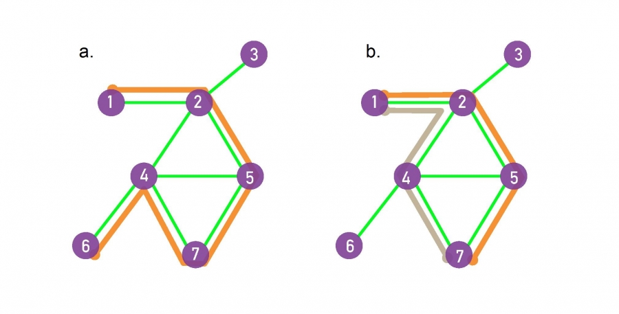
The path shown in orange in (a)
follows the route 1, 2, 5, 7, 4, 6,
hence its length is n = 5.
The shortest paths between nodes 1 and 7,
or the distance d1,7 ,
correspond to one path out of all paths,
with the fewest number of links that connect nodes 1 to 7.
There can be multiple paths of the same length,
as illustrated by the two paths shown in orange and grey.
The network diameter is defined as:
the largest distance in the network,
being dmax = 3 here.
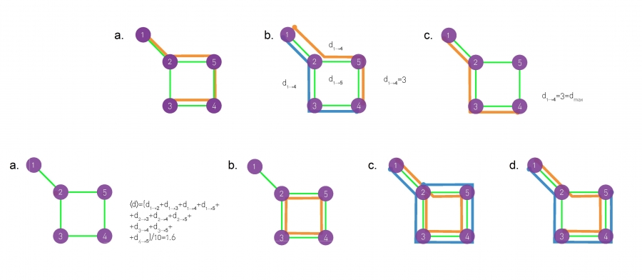
Another example:
path:
A sequence of nodes,
such that each node is connected to the next node,
along the path by a link.
Each path consists of n+1 nodes and n links.
The length of a path is the number of its links,
counting multiple links multiple times.
For example, the orange line 1, 2, 5, 4, 3,
covers a path of length four.
shortest paths:
The path with the shortest distance d between two nodes.
We also call d the distance between two nodes.
Note that the shortest path does not need to be unique:
between nodes 1 and 4 we have two shortest paths,
1, 2, 3, 4 (blue) and
1, 2, 5, 4 (orange),
having the same length d1,4 =3.
diameter (dmax):
The longest shortest path in a graph,
or the distance between the two furthest nodes.
In the graph shown here,
the diameter is between nodes 1 and 4,
hence dmax=3.
The diameter of a network, denoted by dmax,
is the maximum shortest path in the network.
It is the largest distance recorded between any pair of nodes.
average path length
The average of the shortest paths between all pairs of nodes.
For the graph shown on the left we have
<d>=1.6,
whose calculation is shown next to the figure.
cycle:
A path with the same start and end node.
In the graph shown on the left we have only one cycle,
as shown by the orange line.
Eulerian path:
A path that traverses each link exactly once.
The image shows two such Eulerian paths,
one in orange and the other in blue.
Hamiltonian path:
A path that visits each node exactly once.
We show two Hamiltonian paths in orange and in blue.
In an undirected network,
if there is a path between nodes i and j,
then they are defined as connected.
If such a path does not exist,
they are disconnected,
in which case we have dij = inf.
A network itself is defined as connected,
if all pairs of nodes in the network are connected.
A network is defined as disconnected,
if there is at least one pair with dij = inf.
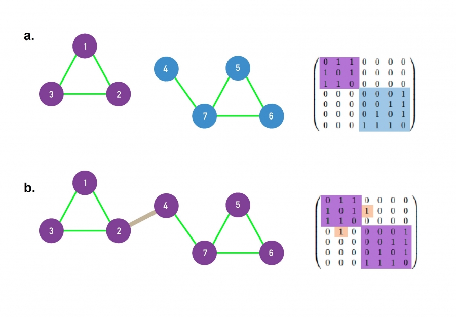
A small network consisting of two disconnected
components.
There is a path between any pair of nodes in the (1,2,3)
component,
as well in the (4,5,6,7) component.
There are no paths between nodes that belong to the different
components.
The right panel shows the adjacently matrix of the network.
If the network has disconnected components,
the adjacency matrix can be rearranged into a block diagonal form,
such that all nonzero elements of the matrix,
are contained in square blocks along the diagonal of the matrix,
and all other elements are zero.
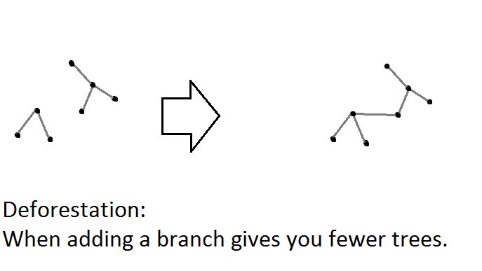
The addition of a single link, called a bridge, shown in
grey,
turns a disconnected network into a single connected
component.
Now there is a path between every pair of nodes in the network.
Consequently, the adjacency matrix cannot be written in a block diagonal
form.
There exist a number of algorithms for identifying connected components from a matrix.
https://en.wikipedia.org/wiki/Clustering_coefficient
Recall: a neighbor is an adjacent node.
First, we define a clustering coefficient for a single node.
The clustering coefficient statistic for a particular node
captures:
the degree to which the neighbors of a given node link to each
other.
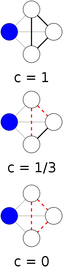
For a node i with degree ki the local clustering coefficient
is defined as:
\(C_i = \frac{{2L_i }}{{k_i \left( {k_i - 1}
\right)}}\)
where Li represents the number of links between the
ki neighbors of node i.
Ci for a given node is between 0 and 1.
If none of the neighbors of node i link to each other, then:
Ci = 0.
If the neighbors of node i form a complete graph, then:
Ci = 1. i.e. they all link to each other.
Ci is the probability that two neighbors of a node link to
each other.
Consequently, C = 0.5 implies that:
there is a 50% chance that two neighbors of a node are linked.
A node-wise Ci for every node,
provides an overview of the network’s local link density.
The more densely interconnected the neighborhood of node i,
the higher is its local clustering coefficient.
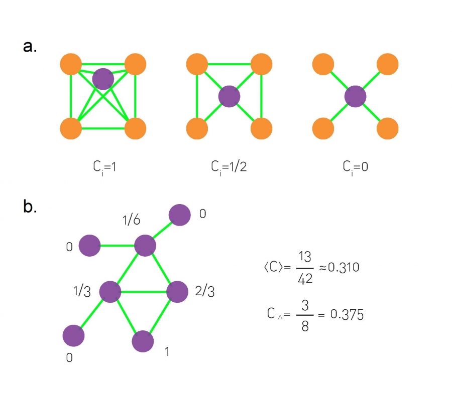
Clustering coefficients:
The local clustering coefficient, \(C_i\), of the central node with degree
\(k_i = 4\),
for three different configurations of its neighborhood.
The local clustering coefficient measures the local density of links in
a node’s vicinity.
A small network, with the local clustering coefficient of each
nodes shown next to it.
We also list the network’s average clustering coefficient
<C>,
and its global clustering coefficient \(C_{\delta}\).
Note that for nodes with degrees ki = 0,1, the clustering coefficient is
zero.
The degree of clustering of a whole network is captured by the
average clustering coefficient,
<C>, representing the average of Ci over all nodes i
= 1, …, N
Mean clustering coefficient of the graph is defined as:
the mean of that of all nodes:
\(\left\langle C \right\rangle =
\frac{1}{N}\sum\limits_{i = 1}^N {C_i }\)
These are statistics intended to capture an real phenomenon.
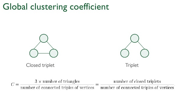
Another way to define a global graph-wide clustering coefficient is
defined as:
the number of closed triplets, or 3 x triangles,
over the total number of triplets (both open and closed).
https://en.wikipedia.org/wiki/Scale-free_network
https://en.wikipedia.org/wiki/Small-world_network
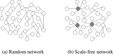
Scale free (power) versus random (normal skewed)
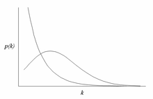
Recall: p(k) is proportion of nodes with that k.
We can view different types of networks by their degree and clustering
coefficient.
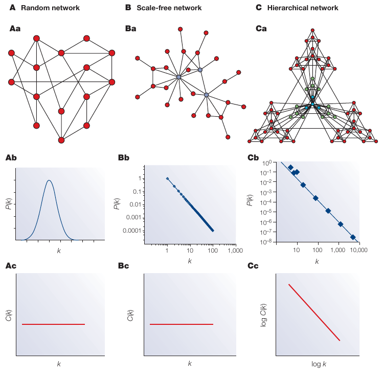
A real network, the central metabolism of Escherichia coli
C is nodewise clustering coefficient distribution.
k is nodewise degree distribution.
d | The degree distribution,
P(k) of the metabolic network illustrates its scale-free topology.
e | The scaling of the clustering coefficient C(k),
with the degree k illustrates the hierarchical architecture of
metabolism.
The data shown in d and e represent an average over 43 organisms.
f | The flux distribution follows a power law,
which indicates that most reactions have small metabolic flux,
whereas a few reactions, with high fluxes,
carry most of the metabolic activity.
This plot is based on data that was collected by Emmerling et
al. 106.
It should be noted that on all three plots,
the axis is logarithmic,
and a straight line on such log-log plots indicates a power-law
scaling.
CTP, cytidine triphosphate;
GLC, aldo-hexose glucose;
UDP, uridine diphosphate;
UMP, uridine monophosphate;
UTP, uridine triphosphate.
https://en.wikipedia.org/wiki/Preferential_attachment
The origin of the scale-free topology and hubs in biological
networks,
can be reduced to two basic mechanisms,
growth and preferential attachment.
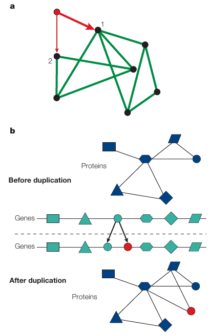
Growth means that the network structure emerges over time,
through the subsequent addition of new nodes,
such as the new red node that is added to the network,
that is shown in part a.
Preferential attachment means that:
new nodes prefer to link to more connected nodes.
For example,
the probability that the red node will connect to node 1,
is twice as large as connecting to node 2,
as the degree of node 1 (k1=4),
is twice the degree of node 2 (k2=2).
Growth and preferential attachment generate hubs,
through a ‘rich-gets-richer’ mechanism:
The more connected a node is,
the more likely it is that new nodes will link to it,
which allows the highly connected nodes to acquire new links,
faster than their less connected peers.
In protein interaction networks,
scale-free topology seems to have its origin in gene duplication.
Small protein interaction network (blue),
and the genes that encode the proteins (green).
When cells divide, occasionally one or several genes are copied
twice,
into the offspring’s genome
(illustrated by the green and red circles).
This induces growth in the protein interaction network,
because now we have an extra gene that encodes a new protein (red
circle).
The new protein has the same structure as the old one,
so they both interact with the same proteins.
The proteins that interacted with the original duplicated protein,
will each gain a new interaction to the new protein.
Proteins with a large number of interactions,
tend to gain links more often,
as it is more likely that they interact with the duplicated
protein.
This mechanism generates preferential attachment in cellular
networks.
In the example in part b,
it does not matter which gene is duplicated,
the most connected central protein (hub) gains one interaction.
In contrast, the square, which has only one link,
gains a new link only if the hub is duplicated.
Is this broader than graph theory?
Rich get richer?
Conglomeration observed in scales:
countries, industries, etc.
https://en.wikipedia.org/wiki/The_rich_get_richer_and_the_poor_get_poorer
https://en.wikipedia.org/wiki/Scale-free_network#Generative_models
https://en.wikipedia.org/wiki/Wealth_concentration
Agglomeration and conglomeration emerge upwards.
We can define simplistic graph elements,
and then quantify the number of them.
We did this with a second definition of clustering above.
The scale-free and hierarchical features of complex networks,
emphasize organizing principles,
that determine the network’s large-scale structure.
An alternative approach starts from the bottom,
and looks for highly representative patterns of interactions,
that characterize specific networks.
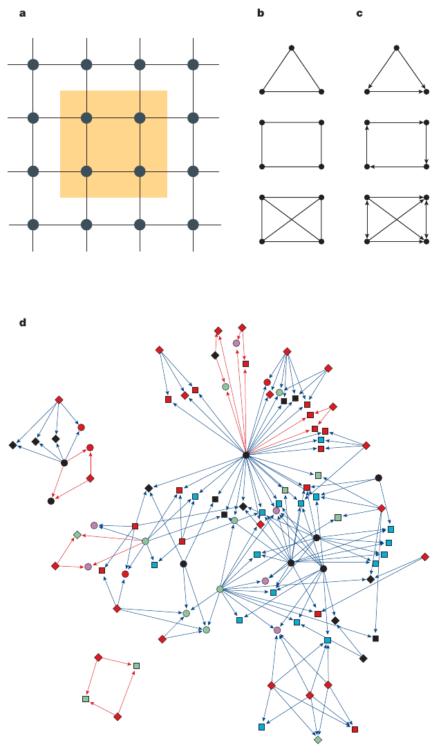
Subgraphs
A connected subgraph represents a subset of nodes,
that are connected to each other in a specific wiring diagram.
For example, in part a of the figure above,
nodes that form a little square (yellow),
represent a subgraph of a square lattice.
Networks with a more intricate wiring diagram,
can have various different subgraphs.
Examples of different potential subgraphs,
that are present in undirected networks,
are shown in part b of the figure.
A directed network is shown in part c.
The number of distinct subgraphs grows exponentially,
with an increasing number of nodes.
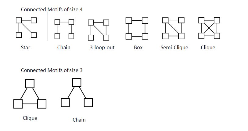
Motifs
Not all subgraphs occur with equal frequency.
Indeed, the square lattice (see figure, part a),
contains many squares, but no triangles.
In a complex network with an apparently d random wiring diagram,
all subgraphs, from triangles to squares and pentagons and so on, are
present.
However, some subgraphs, which are known as motifs,
are over represented as compared to a randomized version of the same
network.
The directed triangle motif that is known as the feed-forward
loop,
(see figure, top of part c),
emerges in both transcription-regulatory and neural networks,
whereas four-node feedback loops (see figure, middle of part c)
represent characteristic motifs in electric circuits,
but not in biological systems.
To identify the motifs that characterize a given network,
all subgraphs of n nodes in the network are determined.
Next, the network is randomized while keeping the number of nodes,
links and the degree distribution unchanged.
Subgraphs that occur significantly more frequently in the real
network,
as compared to randomized one,
are designated to be the motifs.
Motif clusters
Motifs and subgraphs that co-occur in a given network are not
independent of each other.
For the Escherichia coli transcription-regulatory,
in part d of the figure, all of the 209 bi-fan motifs
(a motif with 4 nodes) that are found in the network are shown.
As the figure shows,
208 of the 209 bi-fan motifs form two extended motif clusters,
and only one motif remains isolated (bottom left corner).
Such clustering of motifs into motif clusters,
seems to be a general property of all real networks.
In part d of the figure,
the motifs that share links with other motifs,
are shown in blue;
otherwise they are red.
The different colours and shapes of the nodes,
illustrate their functional classification.
https://en.wikipedia.org/wiki/Centrality
In graph theory and network analysis,
indicators of centrality identify important vertices within a
graph.
Example applications include identifying the most:
influential person(s) in a social network,
key infrastructure nodes in the Internet or urban networks,
super-spreaders of disease, etc.
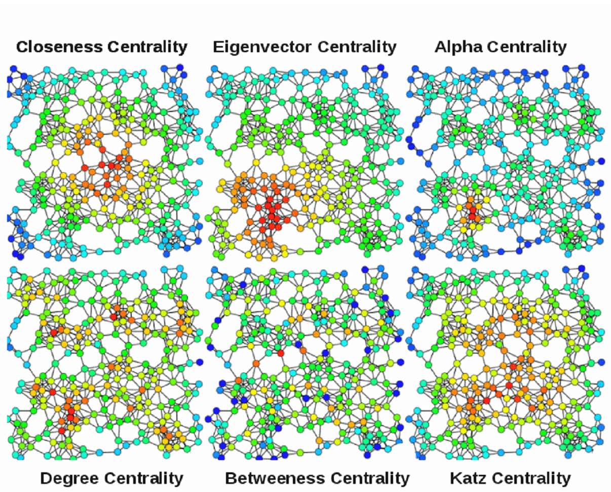
Degree centrality is just degree
Betweenness centrality gives us another way to think about importance
in a network.
It measures the number of shortest paths in the graph,
that pass through the node divided by the total number of shortest
paths.
This metric computes all the shortest paths between every pair of
nodes,
and sees what is the percentage of that passes through node k.
That percentage gives us the centrality for node k.
Nodes with high betweenness centrality,
control information flow in a network.
Edge betweenness is defined in a similar fashion.
In order to properly define closeness,
we need to define the term farness.
Distance between two nodes is the shortest paths between them.
The farness of a node is:
the sum of distances between that node and all other nodes.
And the closeness of a node is the inverse of its farness.
It is the normalized inverse of the sum of topological distances in the
graph.
The most central node,
is the node that propagates information the fastest through the
network.
The description of closeness centrality makes it similar to the degree
centrality.
Is the highest degree centrality always the highest closeness
centrality?
No. Think of the example where one node connects two components,
that node has a low degree centrality but a high closeness
centrality.
What happens to a graph over time,
when you add or remove edges?
Check out graph data-sets here: ../Content.html
Next: 24-CompEpi.html