Functions

A function is an abstract model of computation:
you give it some input, and it produces a result.

The result is completely determined by the input:
if you repeatedly apply the same function to the same argument,
then you will always obtain the same result.

A function can be described in various ways:
algebraically (a formula),
in programming code (a formula),
numerically (a table),
graphically (a plot), or
in words.

For a numeric table or graph:
For any particular input value x,
a function specifies the value y of the result.

This can be represented as an ordered pair (x, y),
and the entire function is represented as a set of ordered pairs.

This representation of a function is called a function graph,
and it is similar to the digraph used to represent relations.

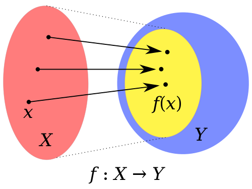
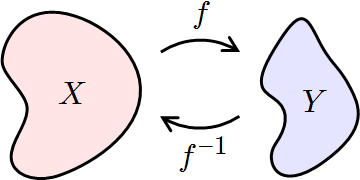
Functions/domain-codomain-image-range.png

A function f from X to Y.
The red oval X is the domain of f.
The blue oval Y is the codomain of f.
The yellow oval inside Y is the image of f.
Sometimes “range” refers to the image, and sometimes to the codomain.

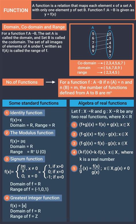
A is called the argument type,
and B is called the result type of the function.
Formally, let A and B be sets.
A function f, with type A → B, is a relation with domain A and codomain B, such that:
∀x ∈ A. ∀y₁ ∈ B. ∀y₂ ∈ B. ((x, y₁) ∈ f ∧ (x, y₂) ∈ f) → y₁ = y₂ .

The definition says that a function is a set of ordered pairs, just like a relation.
The set of ordered pairs is called the graph of the function.
If an ordered pair (x, y) is a member of the function, then x ∈ A and y ∈ B.
Furthermore, the definition states formally that:
if the result of applying a function to an argument x could be y₁,
but it could alternatively be y₂,
then it must be that y₁ = y₂.
This is just a way of saying that:
There is a unique result corresponding to each argument.

An application of the function f to the argument x,
provided that f :: A → B and x :: A,
is written as either f x or as f (x),
and its value is y, if the ordered pair (x, y) is in the graph of f;
otherwise the application of f to x is undefined:
f x = y ↔︎ (x, y) ∈ f

A type can be thought of as the set of possible values,
that a variable might have.
Thus the statement ‘x :: A’,
which is read as ‘x has type A’,
is equivalent to x ∈ A.
The type of the function is written as A → B,
which suggests that the function takes an argument of type A,
and transforms it to a result of type B.
This notation is a clue to an important intuition:
the function is a black box machine that turns arguments into results.

If x ∈ A, and there is a pair (x, y) ∈ f,
then we say that ‘f x is defined to be y’.
However, if x ∈ A but there is no pair (x, y) ∈ f,
we say ‘f x is undefined’.
A shorthand mathematical notation for saying ‘f x is undefined’ is:
f x = ⊥,
where the symbol ⊥ denotes an undefined value.

Some of the elements of types A and B may not actually appear in the function,
in any of the ordered pairs belonging to a function graph.
The subset of type A consisting of arguments,
for which the function is actually defined,
is called the domain of the function.
Similarly, a subset of B,
consisting just of the results that actually can be returned by the function,
is called the image.
These sets are defined formally as follows:

The domain and the image of a function f are defined as:
domain f = {x | ∃y. (x, y) ∈ f}
image f = {y | ∃x. (x, y) ∈ f}

the domain of a function is the set of all x,
such that (x, y) appears in its graph,
while its image is the set of all y,
such that (x, y) appears.

Thus a function is defined for every element of its domain,
and is able to produce every element of its image.

1.2.1 Partial functions

Recall that the domain of a function, f :: A → B,
is a subset of A, consisting of all the elements of A, for which f is defined.

There are two sets that can be used to describe the possible arguments of f .
The argument type A is generally thought of as a constraint:
if you apply f to x,
then it is required that x ∈ A (alternatively, x :: A).

If this constraint is violated,
then the application f x is meaningless.
The domain of f is a set of arguments,
for which f will produce a result.
Naturally, domain f must be a subset of A.
However, there is an important distinction,
between functions where the domain is the same as the argument type,
and functions where the domain is a proper subset of the argument type.

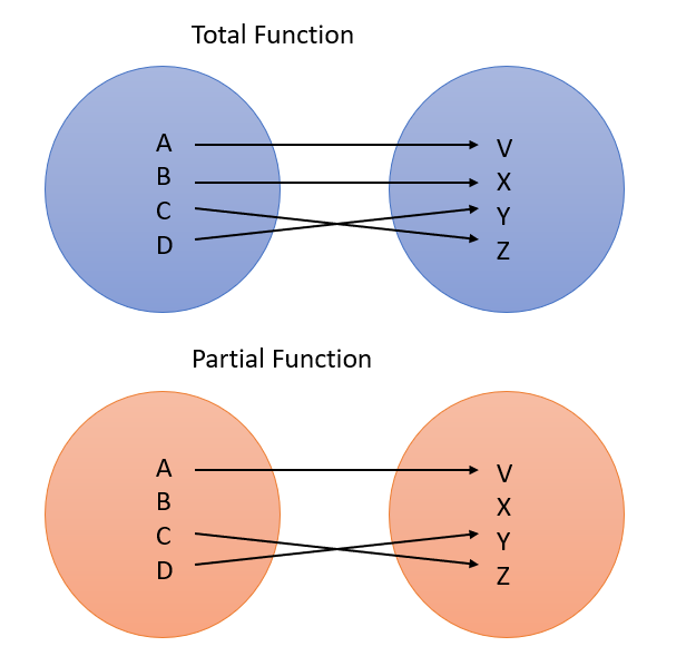
Let f :: A → B be a function.
If the domain is f = A, then f is a total function.
If the domain is f ⊂ A, then f is a partial function.

If f is a partial function, and x ∈ domain f,
then we say that f x is defined.

There are several standard ways to describe an application of f y,
where y :: A, but y /∈ domain f:
It is common, especially in mathematics, to write ‘f y is undefined’.
Another approach, frequently used in theoretical computer science,
is to introduce a special symbol ⊥ (pronounced bottom),
which stands for an undefined value.
This allows us to write:
f y = ⊥

1.2.2 Function composition

It is often possible to structure a computation,
as a sequence of function applications organised as a pipeline:
the output from one function becomes the input to the next, and so on.

In the simplest case, there are just two functions in the pipeline:
the input x goes into the first function, g,
whose output goes into the second function f.

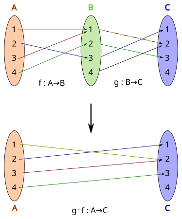
Let g :: a → b, and f :: b → c be functions.
The composition of f with g, written f ◦ g, is a function such that:
(f ◦ g) :: a → c
(f ◦ g) x = f (g x)

When you think of composition as a pipeline,
the input x goes into the first function g;
this produces an intermediate result g x,
which is the input to the second function f,
and the final result is f (g x).

Notice, however, that in the notation f ◦ g,
the functions are written in backwards order.
This may be unfortunate,
but this is the standard definition of function composition,
and you need to be familiar with it.
Just remember that f ◦ g means first apply g, then f.

The ◦ symbol is an operator that takes two functions,
and produces a new function,
just as + is an operator that takes two numbers,
and produces a new number.

The first argument to ◦ is f :: b → c,
and the second argument is g :: a → b,
and the entire composition takes an input, x :: a,
and returns a result (f (g x)) :: c.
Therefore the ◦ operator has the following type:

(.) :: (b -> c) -> (a -> b) -> (a -> c)
(f . g) x = f (g x)

Suppose that you wish to increment the second elements of a list of pairs.
You could write this as:

map increment (map snd [(1,2),(3,4)])
-- Or
map (increment.snd) [(1,2),(3,4)]

Functional composition (◦) is associative.
That is, for all functions:
h :: a → b,
g :: b → c,
f :: c → d,

f ◦ (g ◦ h) = (f ◦ g) ◦ h,
and both the left- and right-hand sides of the equation have type a → d.

Proof.
We need to prove that the two functions,
f ◦ (g ◦ h) and (f ◦ g) ◦ h,
are extensionally equal.
To do this we need to choose an arbitrary x :: a,
and show that both functions give the same result when applied to x.
That is, we need to prove that the following equation holds:

This is done by straightforward equational reasoning,
repeatedly using the definition of ◦:

The significance of this theorem is that:
we can consider a complete pipeline as a single black box;
there is no need to structure it two functions at a time.
Similarly, you can omit the redundant parentheses in the mathematical notation.
The following compositions are all identical:

The parentheses in all of these expressions have no effect,
not changing the meaning of the expression,
and they make the notation harder to read,
so it is customary to omit them and write simply:

You must put parentheses around an expression denoting a function,
when you apply it to an argument, for example:

1.2.3 Properties of Functions

We have used four sets to characterise a function:
the argument type, the domain, the result type, and the image.
There are several useful properties of functions,
that concern these four sets,
and we will examine them in this section.

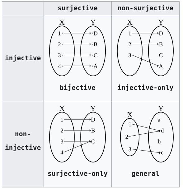
Injections, surjections, and bijections are classes of functions,
distinguished by the manner in which arguments (input expressions from the domain)
and images (output expressions from the codomain)
are related or mapped to each other.

1.2.3.1 Surjective

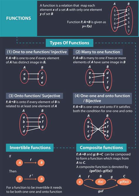
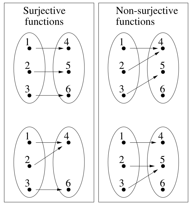
A surjective function has an image,
that is the same as its result type (or range).
Thus the function can, given suitable input,
produce any of the elements of the result type.

not :: Bool -> Bool
member v :: [Int] -> Bool
increment :: Int -> Int
id :: a -> a

All of these functions have result types that are no larger than their domain types.

The following Haskell functions are not surjective.
The length function returns only zero or a positive integer,
and abs returns the absolute value of its argument,
so both functions can never return a negative number.
The times two function may be applied to an odd or an even number,
but it always returns an even result.

length :: [a] -> Int
abs :: Int -> Int
times_two :: Int -> Int

The composition of two injections is again an injection,
but if g ∘ f is injective,
then it can only be concluded that f is injective,
as in the figure immediately above.

1.2.3.2 Injective

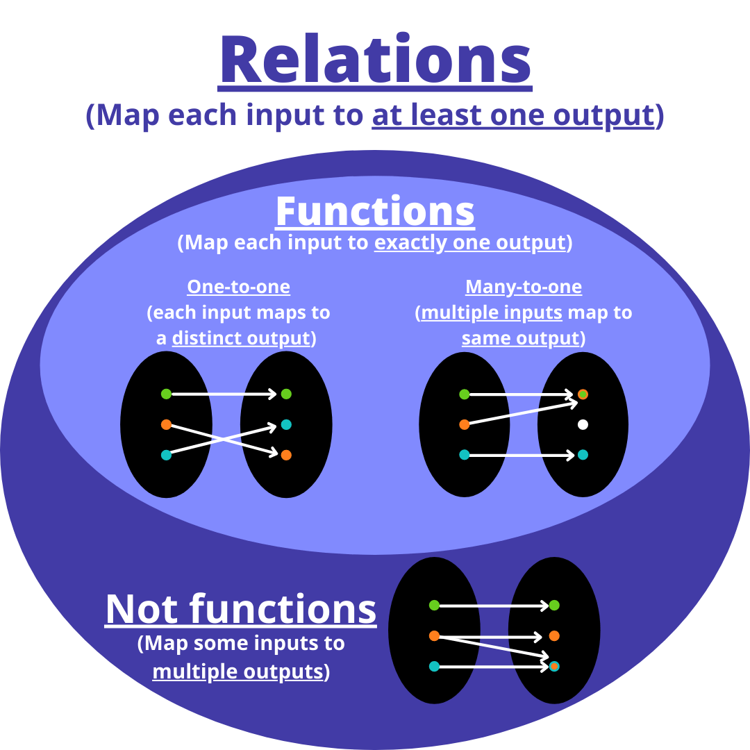
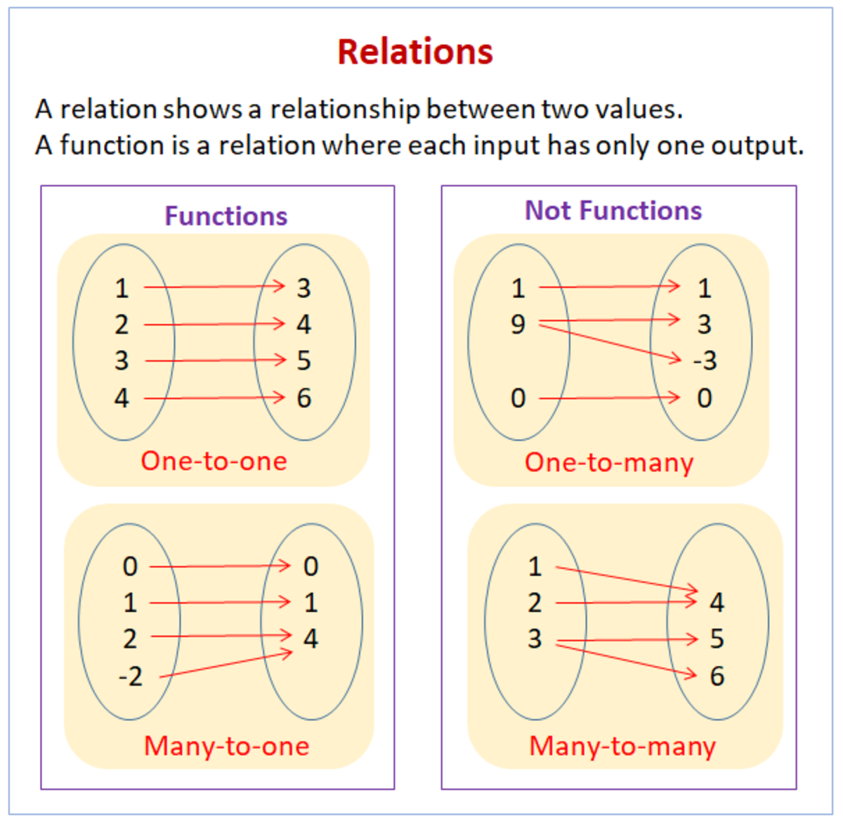
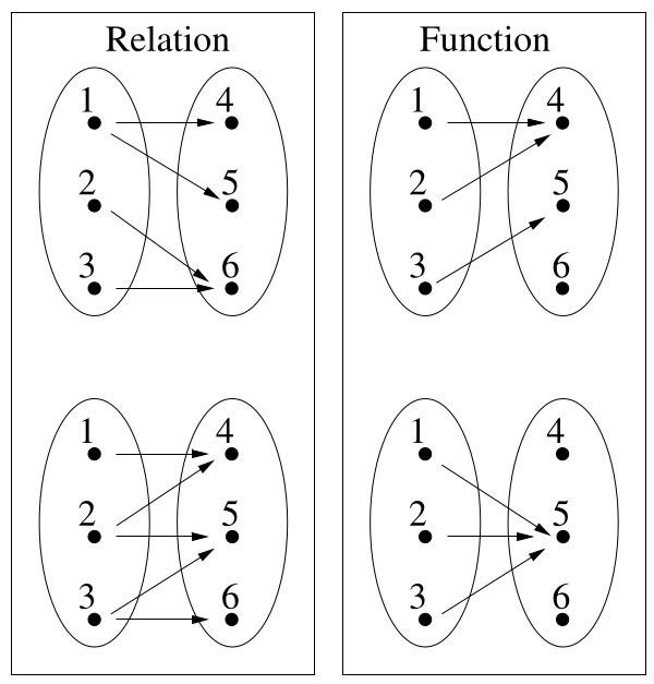
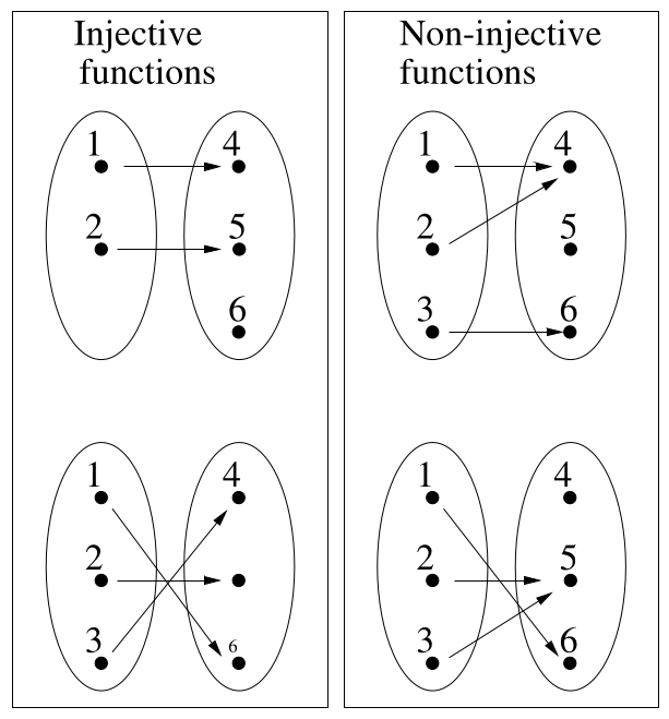
The essential requirement that a relation must satisfy, in order to be a function,
is that it maps each element of its domain,
to exactly one element of the image.
An injective function has a similar property:
each element of the image, is the result of applying the function,
to exactly one element of the domain.

The function f :: A → B is injective if:
∀a,a' ∈ A. a /= a' → f a /= f a'

(/\) True :: Bool -> Bool
increment :: Int -> Int
id :: a -> a
times_two :: Int -> Int

The following Haskell functions are not injective.
The length function is not injective,
because it will map both [1,2,3] and [3,2,1] to the same number, 3.
There are infinitely many other examples that would suffice,
to show that length is not injective,
but you only have to give one.
The function take n is not injective,
because it will map both [a₁, a~2, …, a_n, x] and [a₁, a₂, …, a~n, y],
to the same result [a₁, a₂, …, a~n], even if x /= y.

length :: [a] -> Int
take n :: [a] -> [a]

The composition of two injections is again an injection,
but if g ∘ f is injective,
then it can only be concluded that f is injective,
as in the figure immediately above.

1.2.3.3 Bijective

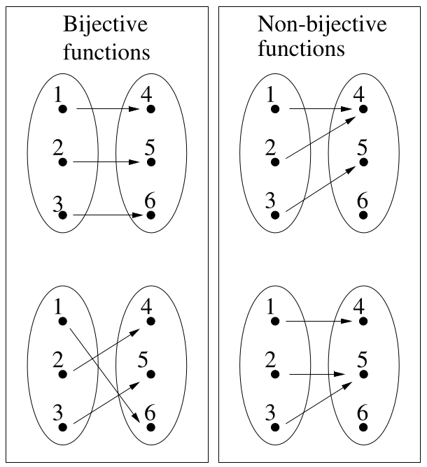
A function is bijective if it is both surjective and injective.
An alternative name for ‘bijective’ is one-to-one and onto.
A bijective function is sometimes called a one-to-one correspondence.

The domain and image of a bijective function must have the same number of elements.
This is stated formally in the following theorem:

Proof.
Suppose that the domain A is larger than the image B.
Then f cannot be injective, by the Pigeonhole Principle (below).
Now suppose that B is larger than A.
Then not every element of B can be paired with an element of A:
there are too many of them, so f cannot be surjective.
Thus a function is bijective, only when its domain and image are the same size.

A bijective function must have a domain and image that are the same size,
and it must also be surjective and injective.
As before, we assume that these functions are finite.

The composition of two bijections is again a bijection,
but if g ∘ f is a bijection,
then it can only be concluded that f is injective and g is surjective
(see the figure at right immeditaely above).

1.2.3.4 Permutations

A permutation must minimally be a bijective function f :: A → A;
i.e., it must have the same domain and image.
The only thing a permutation function can do is to shuffle its input;
it cannot produce any results that do not appear in its input.

Sometimes it is convenient to think of a permutation as a function,
that reorders the elements of a list;
this is often simpler and more direct than defining a function on the indices.
For example, it is natural to say that a sorting function has type [a] → [a].
The following definition provides a convenient way to represent a permutation,
as a function that reorders the elements of a list:

A list permutation function is a function f :: [a] → [a],
that takes a list of values,
and rearranges them using a permutation g, such that:
xs !! i = (f xs) !! (g i)

If you rearrange a list of values, and then rearrange them again,
you simply end up with a new rearrangement of the original list,
and that could be described directly as a permutation.
This idea is stated formally as follows:

Let f, g :: A → A be permutations.
Then their composition f ◦ g is necessarily also a permutation.

1.2.3.5 Inverse

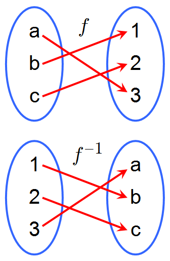
A function f :: A → B takes an argument x :: A and gives the result (f x) :: B.
The inverse of the function goes the opposite direction:
given a result y :: B, it produces the argument x :: A,
which would cause f to yield the result y.

Not all functions have an inverse.
For example, if both (1, 5) and (2, 5) are in the graph of a function,
then there is no unique argument that yields 5.

Let f :: A → B be a bijection.
Then the inverse of f, denoted f₋₁, has type f₋₁ :: B → A,
and its graph is {(y, x) | ∃x, y. (x, y) ∈ f}

1.2.3.6 The Pigeonhole Principle

The Pigeonhole Principle encapsulates a common sense form of reasoning,
about the relationship between two finite sets.
It says that:
if A and B are finite sets, where |A| > |B|,
then no injection exists from A to B.
Since each element of the domain must be assigned a pigeonhole in the image,
and the domain is bigger than the image,
then there must be an element left over,
because at most one pigeon fits in a pigeonhole.
This principle is frequently used in set theory proofs,
especially proofs of theorems about functions.
There are a variety of ways in which to state the pigeonhole principle formally.

Let A and B be finite sets,
such that |A| > |B| and |A| > 1.
Let f :: A → B, then:

1.2.4 Cardinality of Sets and Counting

One of the most fundamental properties of a set is its size,
and this must be defined carefully,
because of the subtleties of infinite sets.
Bijections are a crucial tool for reasoning about the sizes of sets.

A bijection is often called a one-to-one correspondence,
which is a good description:
if there is a bijection f :: A → B,
then it is possible to associate each element of A,
with exactly one element of B, and vice versa.

This is really what you are doing when you count a set of objects:
you associate 1 with one of them, 2 with the second, and so on.
When you have associated all the objects with a number,
then the number n associated with the last one is the number of objects.

If there is a bijection f :: {1, 2, …, n} → S.
the number of objects in S is n.
This idea is used formally to define the size of a set,
which is called its cardinality:

A set S is finite, if and only if, there is a natural number, n,
such that there is a bijection mapping the natural numbers {0, 1, …, n − 1} to S.
The cardinality of S is n, and it is written as |S|.

In other words, if S is finite, then it can be counted,
and the result of the count is its cardinality
(i.e., the number of elements it contains).

We would also like to define what it means to say that a set is infinite.
It would be meaningless to say:
“a set is infinite if the number of elements is infinity”,
because infinity is not a natural number.
We need to find a more fundamental property,
that distinguishes infinite sets from finite ones.

A set A is infinite, if there exists an injective function f :: A → B,
such that B is a proper subset of A.
We can use the properties of a function over a finite domain A, and result type B,
to determine their relative cardinalities:

If f is a surjection, then |A| ≥ |B|.
If f is an injection, then |A| ≤ |B|.
If f is a bijection, then |A| = |B|.

Earlier we discussed counting the elements of a finite set,
placing its elements in a one-to-one correspondence with the elements of {1, 2, …, n}.
Even though there is no natural number, n,
which is the size of an infinite set,
we can use a similar idea to define what it means to say that,
two sets have the same size, even if they are infinite:

If there is a bijection f :: A → B,
then two sets A and B have the same cardinality,

A set is countable, if it has the same cardinality as the set of natural numbers.
In daily life, we use the word counting to describe the process of enumerating a set,
with 1, 2, 3, …, so it is natural to call a set countable,
if it can be enumerated, even if the set is infinite.

1.2.4.1 Example: Rationals are countable

It turns out that some infinite sets are countable,
and others are not, as we will see shortly.
In computer science applications,
it is particularly important to know whether an infinite set is countable,
since a computer performs a sequence of operations that is countable.
It is often possible for a computer to print out the elements of a countable set;
it will never finish printing the entire set,
but any specific element will eventually be printed.
However, if a set is not countable,
then the computer will not even be able to ensure that a given element will eventually be printed.

A rational number is a fraction of the form x/y,
where x and y are integers.
We can represent a ratio as a pair of integers,
the first being the numerator and the second the denominator.

Now suppose that we want to enumerate all of these ratios:
we need to put them into one-to-one correspondence with N.
Our goal is to create a series of columns,
each of which has an index n indicating its place in the series.
A column gives all possible fractions with n as the numerator:

Every line in this sequence is finite,
so it can be printed completely before the next line is started.
Each time a line is printed,
progress is made on all of the columns and a new one is added.
Every ratio will eventually appear in the enumeration.
Thus the set Q of rational numbers can be placed in one-to-one correspondence with N,
and Q is countable.

1.2.4.2 Example: The Real Numbers Are Uncountable

Obviously, if A ⊆ B, then we cannot say that:
set B is larger than set A, since they might be equal.
Surprisingly, even if we know that A is a proper subset of B, A ⊂ B,
then we still cannot say that B has more elements:
as the previous section demonstrated,
it is possible that both are infinite but countable.
For example, the set of even numbers is a proper subset of the set of natural numbers,
yet we say that both sets have the same cardinality!

It turns out that some infinite sets are not countable.
Such a set is so much bigger than the set of natural numbers,
that there is no possible way to make a one-to-one correspondence,
between it and the naturals.
The set of real numbers has this property.
In this section we will explain why,
and introduce a technique called diagonalisation,
which is useful for showing that one infinite set has a larger cardinality than another.

We will not give a formal definition of the set of real numbers,
but will simply consider a real number to be a string of digits.
Consider just the real numbers x such that 0 ≤ x < 1;
these can be written in the form .d0 d1 d2 d3 …
There is no limit to the length of this string of digits.

Now, suppose that there is some clever way to place the set of real numbers,
into a one-to-one correspondence with the set of natural numbers
(that is, suppose the set of reals is countable).
Then we can make a table, where the ith row contains the ith real number x_i,
and it contains the list of digits comprising x_i.
Let us name the digits in that list d_i,0 d_i,1 d_i,2 …
Thus d_i,j means the jth digit in the decimal representation of the ith real number x_i.
Here, then, is the table which, attempts to contain a complete enumeration of the set of real numbers:

.d₀₀ d₀₁ d₀₂ d₀₃ …
.d₁₀ d₁₁ d₁₂ d₁₃ …
.d₂₀ d₂₁ d₂₂ d₂₃ …
… … … …

Now we are going to show that this list is incomplete,
by constructing a new real number y,
which is definitely not in the list.
This number y also has a decimal representation,
which we will call .d_y0 d_y1 d_y2 …
Now we have to ensure that y is different from x₀,
and it is sufficient to make the 0th digit of y (i.e., d_y0)
different from the corresponding digit of x0 (i.e., d₀₀).
We can do this by defining a function different :: Digit → Digit.
There are many ways to define this function; here is one:

different x = 
 | x /= 0 = 0
 | x == 0 = 1

It doesn’t matter exactly how different is defined,
as long as it returns a digit that is different from its argument.
We need to ensure that y is different from x_i for every i ∈ N, not just for x₀.
This is straightforward:
just make the ith digit of y different from the ith digit of x_i:

Now we have defined a new number y;
it is real, since it is defined by a sequence of digits,
and it is different from xi for any i.
Furthermore, our construction of y did not depend on knowing how the enumeration of x_i worked:
for any alleged enumeration whatsoever of the real numbers,
our construction will give a new real number that is not in that list.
The conclusion, therefore, is that it is impossible to set up a one-to-one correspondence,
between the set R of reals and the set N of naturals.
R is infinite and uncountable.

1.3 Computer program functions

The ‘function as a graph’ idea used to model a function mathematically is different,
when compared to a function written in a programming language,
although both are realisations of the same idea.
The difference is that:
a set of ordered pairs specifies only what result should be produced for each input;
there is no concept of an algorithm that can be used to obtain the result.
The function graph approach hard-codes the answers.
In contrast, a function in a programming language is represented solely by the algorithm,
and the only way to determine the value of f x is to execute the algorithm on input x.

A programming language function is a method for computing results;
a mathematical function is a set of answers.

Besides providing a method for obtaining the result,
a programming language function has a behaviour:
it consumes memory and time in order to compute the result of an application.
For example, we might write two sorting functions,
one that takes very little time to run on a given test sample and one that takes a long time.
We would regard them as different algorithms,
and would focus on that difference as being important.
The graph model of a function lacks any notion of speed,
and would make no distinction between the two algorithms,
as long as they always produce the same results.

1.3.1 State

A function always returns the same result, given the same argument.
This kind of repeatability is essential:
if √4 = 2 today, then √4 = 2 also tomorrow.
Some computations do not have this property.
For example, many programming languages provide a ‘function’,
that returns the current date and time of day,
and the result returned from such a query will definitely be different tomorrow.
The entire set of circumstances that can affect the result of a computation is called the state.

It is possible to describe computations with state using pure mathematical functions.
The idea is to include the state of the system as an extra argument to the function.
For example, suppose we need a function f,
that takes an integer and returns an integer,
but the result might also depend on the state of the computer system
(perhaps the time of day, or the contents of the file system).
We can handle this by defining a new type State,
that represents all the relevant aspects of the system state,
and then providing the current state to f:

f :: State -> Int -> Int

Now f can return a result that depends on the time of day,
even though it is a mathematical function.
Given the same system state and the same argument,
it will always return the same result.

Programs that need to manipulate the state can be written as pure functions,
with the state made explicit and passed as an argument to each function that uses it.
When a program needs to use the state frequently,
however, it becomes awkward to use explicit State arguments;
this clutters up the program,
and errors in keeping track of the state can be hard to find.

Imperative languages solve this problem by making the state implicit,
and allowing side effects to modify the state.
This is a simple way to allow algorithms to use the system state.
The cost of this approach is that reasoning about the program is more difficult.
In mathematics, if you have an equation of the form x = y,
then you can replace x by y, or vice versa.
This is called substituting equals for equals or equational reasoning.
Unfortunately, equational reasoning doesn’t work in general in imperative languages.
If a function f depends on the system state,
then it is not even true that f x = f x.

1.3.2 Higher Order Functions

A first order function has ordinary (non-function) arguments and result.
A higher order function is one that either takes a function as an argument,
or returns a function as its value, or both.

Example: map
The Haskell function map is a higher order function,
because its first argument is a function,
which map will apply to each element of the second argument,
which is a list.
The type of map is:

map :: (a->b) -> [a] -> [b]

This type reveals that the function is higher order,
since the first argument has a type that contains an arrow,
indicating that this argument is a function.

Example: length
The length function is not higher order.
As its type makes plain,
the argument is a list type and the result is an integer:

length :: [a] -> Int

1.3.2.1 Functions That Take Functions as Arguments

Any function that takes another function as an argument is higher order.
This kind of higher order function will have a type something like the following:
f :: (··· → ···) → ···
We have already seen many examples of such functions in Haskell;
map and foldr are typical.
Generally, this variety of higher order function will also take a data argument,
and it will apply its function argument to its data argument in a special way.

1.3.2.2 Functions That Return Functions

Any function that returns another function as its result is higher order,
and its type will have the following form:
f :: ··· → (··· → ··· )

1.3.3 Multiple inputs and outputs

1.3.3.1 Input tuples

Technically, a function (in either mathematics or Haskell) behave the same,
they takes exactly one argument and returns exactly one result.
There are two ways to get around this restriction.
One method is to package multiple arguments (or multiple results) in a tuple.
Suppose that a function needs two data values, x and y.
The caller of the function can build a pair (x, y) containing these values,
and that pair is now a single object which can be passed to the function.

1.3.3.2 Output tuples

A function must return exactly one result,
but sometimes in practice we want one to return several pieces of information.
In such cases, the multiple pieces can be packaged into a tuple,
and the function can return that as a single result.
This technique is analogous to passing several arguments as a tuple.

1.3.3.3 Currying: partial application

Higher order functions provide another method for passing several arguments to a function.
Suppose that a function needs to receive two arguments, x :: a and y :: b,
and it will return a result of type c.
The idea is to define the function with type:

f :: a → (b → c)
which is equal to:
f :: a → b → c
In Haskell, the → is right-associative in it’s order of operations.

Thus f takes only one argument, which has type a,
and it returns a function with type b → c.
The result function is ready to be applied to the second argument, of type b,
whereupon it will return the result with type c.
This method is called Currying, in honour of the logician Haskell B. Curry
(for whom the programming language Haskell is also named).

The graph of f is a set of ordered pairs;
the first element of each pair is a data value of type a,
while the second element is the function graph for the result function.
That function graph contains, in effect,
the information that f obtained from the first argument.

addInt :: Int -> Int -> Int
addInt x y = x + y

add3 :: Int -> Int
add3 y = 3 + y

3plus5 :: Int
3plus5 = add3 + 5

1.4 Code

-- # Software Tools for Discrete Mathematics
module Stdm11Functions where

import Stdm06LogicOperators
import Stdm08SetTheory
import Stdm10Relations

-- # Chapter 11.  Functions

-- This is the type of image of input under f.
data FunVals a = Undefined | Value a
  deriving (Eq, Show)

-- | This is Fun!
-- >>> isFun [1,2,3] [4,5,6] [(1,Value 4),(2,Value 5),(3,Value 6)]
-- True

-- | This is not Fun...
-- >>> isFun [1,2,3] [4,5,6] [(1,Value 4),(1,Value 5),(1,Value 6)]
-- False
isFun ::
  (Eq a, Eq b, Show a, Show b) =>
  Set a ->
  Set b ->
  Set (a, FunVals b) ->
  Bool
isFun f_domain f_codomain fun =
  let actual_domain = domain fun
   in normalForm actual_domain
        /\ setEq actual_domain f_domain

-- |
-- >>> isPartialFunction [1,2,3] [2,3] [(1,Value 2),(2,Value 3),(3,Undefined)]
-- True

-- |
-- >>> isPartialFunction [1,2] [2,3] [(1,Value 2),(2,Value 3)]
-- False
isPartialFunction ::
  (Eq a, Eq b, Show a, Show b) =>
  Set a ->
  Set b ->
  Set (a, FunVals b) ->
  Bool
isPartialFunction f_domain f_codomain fun =
  isFun f_domain f_codomain fun
    /\ elem Undefined (codomain fun)

-- Some functions to compose below:
fun1 = [(1, Value 2), (3, Value 6), (3, Value 5)]
fun2 = [(2, Value 4), (6, Value 9), (7, Value 10)]

-- |
-- >>> functionalComposition fun1 fun2
-- [(1,Value 4),(3,Value 9)]
functionalComposition ::
  (Eq a, Eq b, Eq c, Show a, Show b, Show c) =>
  Set (a, FunVals b) ->
  Set (b, FunVals c) ->
  Set (a, FunVals c)
functionalComposition f1 f2 =
  normalizeSet [(a, c) | (a, Value b) <- f1, (b', c) <- f2, b == b']

-- | Helper for isSurjective
-- >>> imageValues (codomain [(1, Value 4), (2, Value 5), (3, Value 4)])
-- [4,5,4]
imageValues :: (Eq a, Show a) => Set (FunVals a) -> Set a
imageValues f_codomain = [v | (Value v) <- f_codomain]

-- |
-- >>> isSurjective [1,2,3] [4,5] [(1, Value 4), (2, Value 5), (3, Value 4)]
-- True

-- |
-- >>> isSurjective [1,2,3] [4,5] [(1, Value 4), (2, Value 4), (3, Value 4)]
-- False
isSurjective ::
  (Eq a, Eq b, Show a, Show b) =>
  Set a ->
  Set b ->
  Set (a, FunVals b) ->
  Bool
isSurjective f_domain f_codomain fun =
  isFun f_domain f_codomain fun
    /\ setEq f_codomain (normalizeSet (imageValues (codomain fun)))

-- |
-- >>> isInjective [1,2,3] [2,4] [(1,Value 2),(2,Value 4),(3,Value 2)]
-- False

-- |
-- >>> isInjective [1,2,3] [2,3,4] [(1,Value 2),(2,Value 4),(3,Undefined)]
-- True
isInjective ::
  (Eq a, Eq b, Show a, Show b) =>
  Set a ->
  Set b ->
  Set (a, FunVals b) ->
  Bool
isInjective f_domain f_codomain fun =
  let fun_image = imageValues (codomain fun)
   in isFun f_domain f_codomain fun
        /\ normalForm fun_image

-- |
-- >>> isBijective [1,2] [3,4] [(1,Value 3),(2,Value 4)]
-- True

-- |
-- >>> isBijective [1,2] [3,4] [(1,Value 3),(2,Value 3)]
-- False
isBijective ::
  (Eq a, Eq b, Show a, Show b) =>
  Set a ->
  Set b ->
  Set (a, FunVals b) ->
  Bool
isBijective f_domain f_codomain fun =
  isSurjective f_domain f_codomain fun
    /\ isInjective f_domain f_codomain fun

-- |
-- >>> isPermutation [1,2,3] [1,2,3] [(1,Value 2),(2, Value 3),(3, Undefined)]
-- False

-- |
-- >>> isPermutation [1,2,3] [1,2,3] [(1,Value 2),(2, Value 3),(3, Value 1)]
-- True
isPermutation ::
  (Eq a, Show a) => Set a -> Set a -> Set (a, FunVals a) -> Bool
isPermutation f_domain f_codomain fun =
  isBijective f_domain f_codomain fun
    /\ setEq f_domain f_codomain

-- Real numbers countable?

diagonal :: Int -> [(Int, Int)] -> [(Int, Int)]
diagonal stop rest =
  let interval = [1 .. stop]
   in zip interval (reverse interval) ++ rest

-- |
-- >>>
-- 
rationals :: [(Int, Int)]
rationals = foldr diagonal [] [1 ..]

module HL06FCT where

import Data.List

f x = x ^ 2 + 1

list2fct :: (Eq a) => [(a, b)] -> a -> b
list2fct [] _ = error "function not total"
list2fct ((u, v) : uvs) x
  | x == u = v
  | otherwise = list2fct uvs x

fct2list :: (a -> b) -> [a] -> [(a, b)]
fct2list f xs = [(x, f x) | x <- xs]

ranPairs :: (Eq b) => [(a, b)] -> [b]
ranPairs f = nub [y | (_, y) <- f]

listValues :: (Enum a) => (a -> b) -> a -> [b]
listValues f i = (f i) : listValues f (succ i)

listRange :: (Bounded a, Enum a) => (a -> b) -> [b]
listRange f = [f i | i <- [minBound .. maxBound]]

curry3 :: ((a, b, c) -> d) -> a -> b -> c -> d
curry3 f x y z = f (x, y, z)

uncurry3 :: (a -> b -> c -> d) -> (a, b, c) -> d
uncurry3 f (x, y, z) = f x y z

f1 x = x ^ 2 + 2 * x + 1

g1 x = (x + 1) ^ 2

f1' = \x -> x ^ 2 + 2 * x + 1

g1' = \x -> (x + 1) ^ 2

g 0 = 0
g n = g (n - 1) + n

g' n = ((n + 1) * n) / 2

h 0 = 0
h n = h (n - 1) + (2 * n)

k 0 = 0
k n = k (n - 1) + (2 * n - 1)

fac 0 = 1
fac n = fac (n - 1) * n

fac' n = product [1 .. n]

restrict :: (Eq a) => (a -> b) -> [a] -> a -> b
restrict f xs x
  | elem x xs = f x
  | otherwise = error "argument not in domain"

restrictPairs :: (Eq a) => [(a, b)] -> [a] -> [(a, b)]
restrictPairs xys xs = [(x, y) | (x, y) <- xys, elem x xs]

image :: (Eq b) => (a -> b) -> [a] -> [b]
image f xs = nub [f x | x <- xs]

coImage :: (Eq b) => (a -> b) -> [a] -> [b] -> [a]
coImage f xs ys = [x | x <- xs, elem (f x) ys]

imagePairs :: (Eq a, Eq b) => [(a, b)] -> [a] -> [b]
imagePairs f xs = nub [y | (x, y) <- f, elem x xs]

coImagePairs :: (Eq a, Eq b) => [(a, b)] -> [b] -> [a]
coImagePairs f ys = [x | (x, y) <- f, elem y ys]

injective :: (Eq b) => (a -> b) -> [a] -> Bool
injective f [] = True
injective f (x : xs) =
  notElem (f x) (image f xs) && injective f xs

surjective :: (Eq b) => (a -> b) -> [a] -> [b] -> Bool
surjective f xs [] = True
surjective f xs (y : ys) =
  elem y (image f xs) && surjective f xs ys

c2f, f2c :: Int -> Int
c2f x = div (9 * x) 5 + 32
f2c x = div (5 * (x - 32)) 9

succ1 :: Integer -> Integer
succ1 = \x ->
  if x < 0
    then error "argument out of range"
    else x + 1

succ2 :: Integer -> [Integer]
succ2 = \x -> if x < 0 then [] else [x + 1]

pcomp :: (b -> [c]) -> (a -> [b]) -> a -> [c]
pcomp g f = \x -> concat [g y | y <- f x]

succ3 :: Integer -> Maybe Integer
succ3 = \x -> if x < 0 then Nothing else Just (x + 1)

mcomp :: (b -> Maybe c) -> (a -> Maybe b) -> a -> Maybe c
mcomp g f = (maybe Nothing g) . f

part2error :: (a -> Maybe b) -> a -> b
part2error f = (maybe (error "value undefined") id) . f

fct2equiv :: (Eq a) => (b -> a) -> b -> b -> Bool
fct2equiv f x y = (f x) == (f y)

block :: (Eq b) => (a -> b) -> a -> [a] -> [a]
block f x list = [y | y <- list, f x == f y]

module Sol06 where

import Data.Char
import Data.List
import HL06FCT
import SetOrd

-- | 6.10
h' n = n * (n + 1)

-- | 6.11
k' n = n ^ 2

-- 6.16 f{0, 3} = {(0, 3), (3, 2)}, f [{1, 2, 3}] = {2, 4}, f −1 [{2, 4, 5}] = {1, 2, 3}. Here is the code for the checks:

l_0 = [(0, 3), (1, 2), (2, 4), (3, 2)]

f_0 = list2fct l_0

test_1 = fct2list (restrict f_0 [0, 3]) [0, 3]

test_2 = image f_0 [1, 2, 3]

test_3 = coImage f_0 [0, 1, 2, 3] [2, 4, 5]

-- 6.20.2b Given: f : X → Y , A, B ⊆ X.
-- To be proved: f [A ∩ B] ⊆ f [A] ∩ f [B].
-- Proof:
-- Suppose y ∈ f [A ∩ B]. We have to show that y ∈ f [A] ∩ f [B].
-- From y ∈ f [A ∩ B]: ∃x ∈ A ∩ B with f (x) = y.
-- So x ∈ A : f (x) = y, and x ∈ B : f (x) = y.
-- Therefore, y ∈ f [A] and y ∈ f [B], i.e., y ∈ f [A] ∩ f [B].
-- To see that the inclusion cannot be replaced by an equality, consider the function f : {0, 1, 2} → {0, 1} given by f (0) = 0, f (1) = 0, f (2) = 1. For this f we have f [{0, 2}] = f [{1, 2}] = {0, 1} = f [{0, 2} ∩ {1, 2}] = f [{2}] = {1}. Here is an implementation:
l_1 = [(0, 0), (1, 0), (2, 1)]

f_1 = list2fct l_1

-- | 6.23
bijective :: (Eq b) => (a -> b) -> [a] -> [b] -> Bool
bijective f xs ys = injective f xs && surjective f xs ys

-- | 6.24
injectivePairs :: (Eq a, Eq b) => [(a, b)] -> [a] -> Bool
injectivePairs f xs = injective (list2fct f) xs

surjectivePairs :: (Eq a, Eq b) => [(a, b)] -> [a] -> [b] -> Bool
surjectivePairs f xs ys = surjective (list2fct f) xs ys

bijectivePairs :: (Eq a, Eq b) => [(a, b)] -> [a] -> [b] -> Bool
bijectivePairs f xs ys = bijective (list2fct f) xs ys

-- | 6.27
injs :: [Int] -> [Int] -> [[(Int, Int)]]
injs [] xs = [[]]
injs xs [] = []
injs (x : xs) ys =
  concat [map ((x, y) :) (injs xs (ys \\ [y])) | y <- ys]

-- | 6.28
perms :: [a] -> [[a]]
perms [] = [[]]
perms (x : xs) = concat (map (insrt x) (perms xs))
  where
    insrt :: a -> [a] -> [[a]]
    insrt x [] = [[x]]
    insrt x (y : ys) = (x : y : ys) : map (y :) (insrt x ys)

-- 6.32
comp :: (Eq b) => [(b, c)] -> [(a, b)] -> [(a, c)]
comp g f = [(x, list2fct g y) | (x, y) <- f]

-- 6.57
stringCompare :: String -> String -> Maybe Ordering
stringCompare xs ys
  | any (not . isAlpha) (xs ++ ys) = Nothing
  | otherwise = Just (compare xs ys)

-- 6.65
fct2listpart :: (Eq a, Eq b) => (a -> b) -> [a] -> [[a]]
fct2listpart f [] = []
fct2listpart f (x : xs) = xclass : fct2listpart f (xs \\ xclass)
  where
    xclass = x : [y | y <- xs, f x == f y]

1 Functions

1.1 Readings

1.2 Mathematical functions