
Q: What is the most common tree in Silicon Valley?
A: Binary Search Trees!
Discrete Mathematics using a Comptuter (O’Donnell, Hall, Page) Chapter 5
Discrete Mathematics with Applications - Metric Edition (Epp) Chapter 10
The Haskell Road to Logic, Math and Programming (Doets, van Eijck) Chapter 7
https://www.cs.carleton.edu/faculty/dln/book/ch11_graphs-and-trees_2021_September_08.pdf
https://runestone.academy/ns/books/published/ads/chapter_10.html
https://runestone.academy/ns/books/published/ads/s-what-is-a-tree.html
https://runestone.academy/ns/books/published/ads/s-spanning-trees.html
https://runestone.academy/ns/books/published/ads/s-rooted-trees.html
https://runestone.academy/ns/books/published/ads/s-binary-trees.html
https://runestone.academy/ns/books/published/DiscreteMathText/trees10-3.html
https://runestone.academy/ns/books/published/dmoi-4/sec_trees.html
https://en.wikipedia.org/wiki/Tree_(abstract_data_type)
https://en.wikipedia.org/wiki/Tree_(graph_theory)
https://en.wikipedia.org/wiki/Tree_structure

A tree is a non-linear ordered structure.

Trees are upside down in computer science.
Real tree: leaves at the top, root(s) at the bottom.

Computer science tree: root at the top, leave(s) at the bottom.
Trees are composed of nodes and edges.
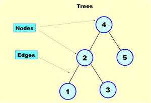
Node is an element in a tree.
Edge is the connection between one node and another.
Widely used abstract data type (ADT),
or data structure implementing the ADT,
that simulates a hierarchical tree structure,
with a root value and subtrees of children with a parent node,
represented as a set of linked nodes.
A (possibly non-linear) data structure,
made up of nodes or vertices and edges,
without having any cycle.
Root at the top, leaves at the bottom:
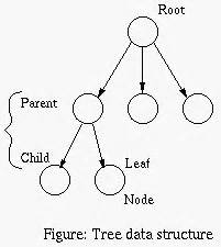
Root is the node at the top of the tree, and has no
parent.
There is only one root per tree and one path from the root node to any
node.
Leaves are bottom nodes without any sub-trees or
children.
They are less commonly called External nodes.
Parents are ancestors of children.
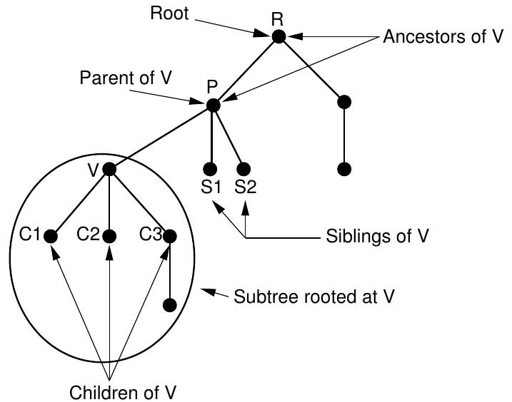
Parent of a node is the single node linked directly
above it.
Any node except the root node has one edge upward to a node called
parent.
Parent is the converse notion of a child.
Child of a node is a node linked directly below
it,
directly connected by its edge downward,
when moving away from the root.
Siblings are an \(n\) group of nodes with the same parent.
Ancestor is any node from which a node descends
directly or indirectly,
which is any node reachable by repeated proceeding from child to
parent.
Descendant is any node that descends from a node
directly or indirectly,
which is any node reachable by repeated proceeding from parent to
child.
If there is a path from \(n_1\) to
\(n_2\),
then \(n_1\) is an ancestor of \(n_2\) and \(n_2\) is a descendant of \(n_1\).
Left and right are defined for nodes and sub-trees
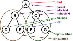
Sub-tree is a smaller tree ‘rooted’ by some
particular node in the tree,
which are descendants of that node.
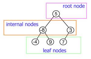
Internal node is a non-root node with at least one child.
Edges are sometimes called branches.
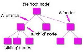
That there are \(n - 1\)
edges follows from the fact that:
each edge connects some node to its parent,
and every node except the root has one parent
If a tree has \(n\) nodes, then it
must have \(n-1\) edges,
as every node is connected to a parent, except for the root.
Trees have levels
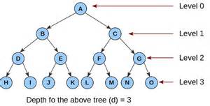
Trees and nodes have depth and height.
Level/depth of a node
represents the familial generation of a node,
or the length of the path from the root to a node.
The level of a node is defined by 1 + (the number of levels between the
node and the root(0)).
If the root node is at level 0,
then its next child node is at level 1,
its grandchild is at level 2, and so on.
In other words, the number of edges from the tree’s root node to the
node.
Level/depth of tree
is length of the longest path from the root to the deepest leaf,
or the maximum depth of any leaf node.
The depth of a tree is equal to the depth of the deepest leaf;
this is always equal to the height of the tree.
height (opposite concept of level/depth) of a node, \(n_i\)
is the length of the longest path from \(n_i\) to a leaf.
Thus all leaves are at height 0.
Height of a tree is equal to the height of the root.
Trees have levels
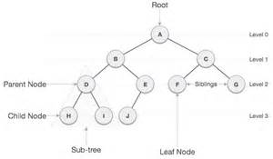
Depth: root is 0; its children are 1, etc.
What is height of these nodes?
Trees have paths:
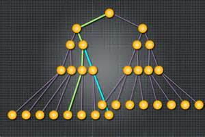
Path is a sequence of nodes and edges connecting a
node with a descendant
(green or blue above for two different leaf nodes).
Only one path from the root to each node.
A path from node \(n_1\) to \(n_k\) is defined as a sequence of
nodes,
\(n_1,\ n_2,\ . . . ,\ n_k\),
such that \(n_i\) is the parent of
\(n_i+1\) for \(1 \leq i < k\).
The length of this path is the number of edges on the path, namely, \(k - 1\).
There is a path of length zero from every node to itself.
With the root is at depth 0, for any node \(n_i\),
the depth of \(n_i\) is the length of
the unique path from the root to \(n_i\) .
Degree of nodes and trees
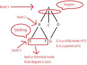
Degree of a node is the number of subtrees of a node.
Degree of a tree is the largest degree of any node in a tree.
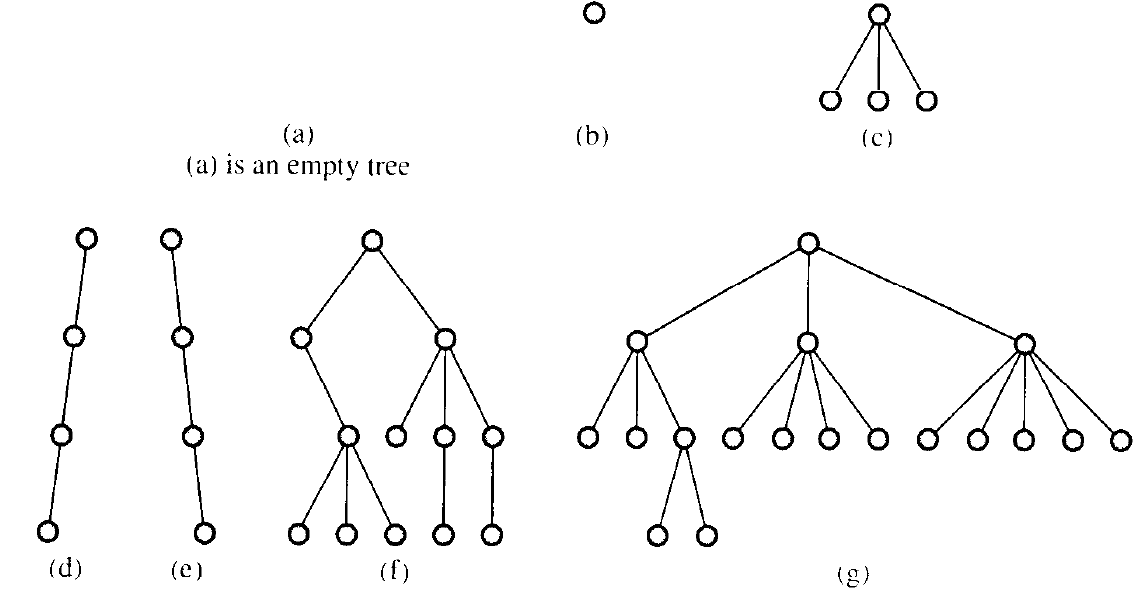
Even single nodes can be considered trees.
Forest is a set of \(n \geq 0\) disjoint trees.
A list is trivially a tree:
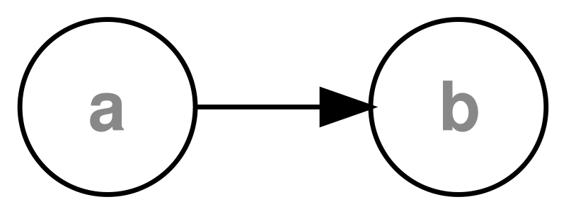
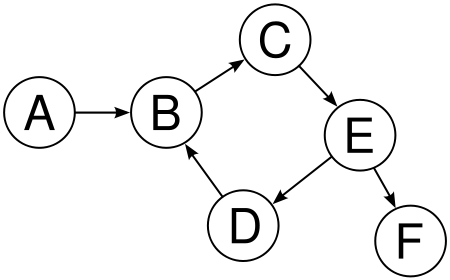

No loops or multi-parent children.
Example tree:
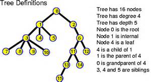
Example tree of characters:
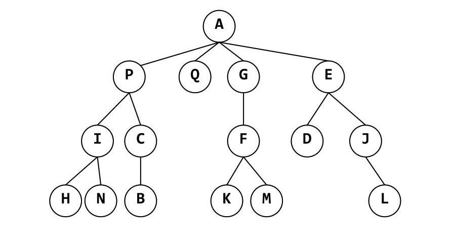
https://en.wikipedia.org/wiki/Binary_tree
Binary trees

Set of nodes is either empty or consists of a node,
called the root together with two binary trees,
called the left and right subtrees,
which are disjoint from each other and from the root;
disjoint means that they have no nodes in common.
Each node has at most two children,
which are referred to as the left child and the right child.
No node can have more than two children.
The depth of an average binary tree is considerably smaller than
N,
the average depth is O(sqrt(N)),
and for a special type of binary tree,
namely the binary search tree,
the average value of the depth is O(log N).
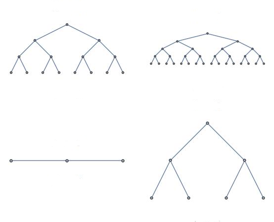
Perfect binary tree:
Binary tree in which all interior nodes have two children,
and all leaves have the same depth or same level.
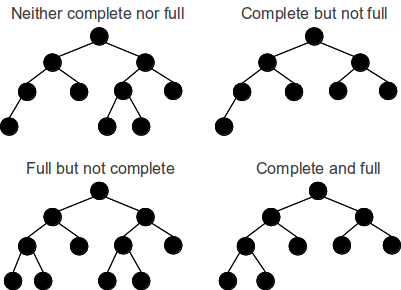
Full (left) and complete (right) binary trees
Full binary tree (left below)
Tree in which every node in the tree has either 0 or 2 children.
Each node in a full binary tree is either:
(1) an internal node with exactly two non-empty children
(2) a leaf.
Complete binary tree (right below)
Has a restricted shape obtained by starting at the root,
and filling the tree by levels from left to right.
Every level, except possibly the last, is completely filled,
and all nodes in the last level are as far left as possible.
The bottom level has its nodes filled in from the left side.
Can be efficiently represented using an array.

Full and complete binary trees

Full and complete binary trees
Balanced binary trees
Has the minimum possible maximum height (a.k.a. depth) for the leaf
nodes,
because for any given number of leaf nodes,
the leaf nodes are placed at the greatest height possible.
One common balanced tree structure is a binary tree structure,
in which the left and right subtrees of every node differ in height by
no more than 1.
One may also consider binary trees where no leaf is much farther away
from the root than any other leaf.
(Different balancing schemes allow different definitions of “much
farther”.)
Degenerate trees:
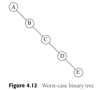
A degenerate (or pathological) tree is where each parent node has
only one associated child node;
performance will behave like a linked list data structure.
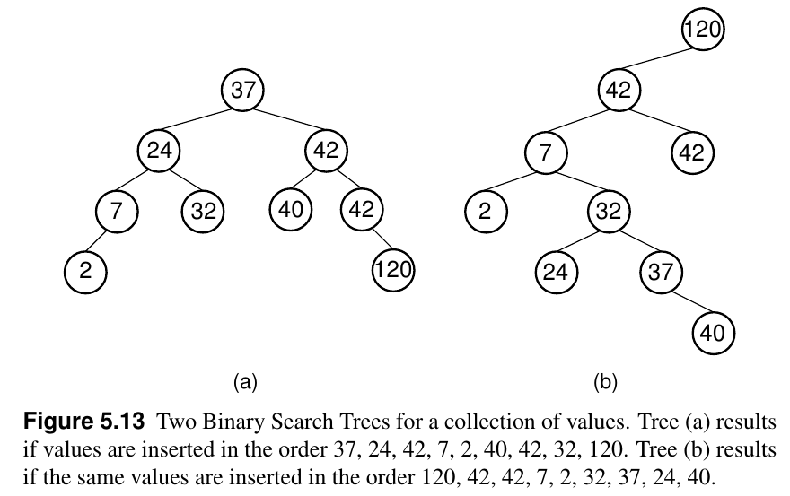
Shape of the binary search tree depends entirely on the order of
insertions and deletions,
and can become degenerate.
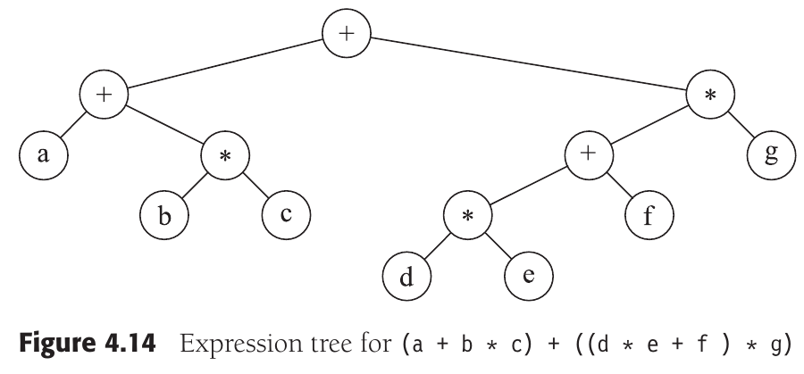
Expression trees:
The leaves are operands, such as constants or variable names, and the other nodes contain operators.
Order of list is obvious, tree not so much.
Any process for visiting all of the nodes in some order is called a
traversal.
Any traversal that lists every node in the tree exactly once is called
an enumeration of the tree’s nodes.
Parents visited before the children.
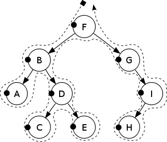
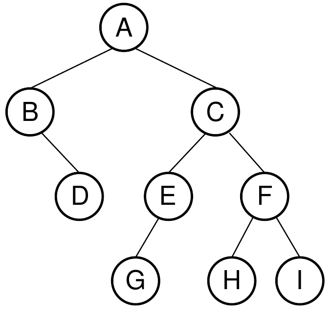
Pre-order: F, B, A, D, C, E, G, I, H
Pre-order Recursive:
Summary:
Pre-order recursive pseudocode algorithm Assuming each node is
referenced to via a pointer called ‘node’, has a left and right
pointer,
and that leaves have two null pointers:
preorder(node)
    if(node == null)
    return
    visit(node)
    preorder(node.left)
    preorder(node.right)
What is the trace on this tree?

Pre-order iterative pseudocode algorithm
iterativePreorder(node)
  if(node == null)
    return
  s = empty stack
  s.push(node)
  while(not s.isEmpty())
    node = s.pop()
    visit(node)
    //right child is pushed first so that
    //left is processed first
    if (node.right != null)
      s.push(node.right)
    if (node.left != null)
s.push(node.left)Children are visited before the parent.

Post-order: A, C, E, D, B, H, I, G, F.
Post-order recursive
Summary:
Post-order recursive pseudocode algorithm Assuming each node is
referenced to via a pointer called ‘node’, has a left and right
pointer,
and that leaves have two null pointers:
postorder(node)
    if(node == null)
    return
    postorder(node.left)
    postorder(node.right)
    visit(node)
What is the trace on this tree?

Post-order iterative pseudocode algorithm
iterativePostorder(node)
  s = empty stack
  lastNodeVisited = null
  while (not s.isEmpty() or node != null)
    if(node != null)
      s.push(node)
      node = node.left
    else
      peekNode = s.peek()
      // if right child exists and traversing node
      // from left child, then move right
      if(peekNode.right != null and
      lastNodeVisited != peekNode.right)
        node = peekNode.right
      else
        visit(peekNode)
lastNodeVisited = s.pop()An inorder traversal first visits the left child (including its
entire subtree),
then visits the node, and finally visits the right child (including its
entire subtree).
Applies to binary trees only.
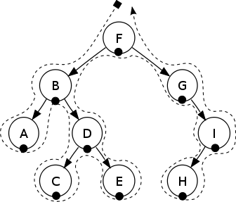
In-order: A, B, C, D, E, F, G, H, I.
In-order: recursive
Why just for binary?
Summary:
In-order:
recursive Assuming each node is referenced to via a pointer called
‘node’,
has a left and right pointer, and that leaves have two null
pointers:
inorder(node)
    if(node == null)
    return
    inorder(node.left)
    visit(node)
    inorder(node.right)
What is the trace on this tree?

In-order: iterative
iterativeInorder(node)
  s = empty stack
  while(not s.isEmpty() or node != null)
    if(node != null)
      s.push(node)
      node = node.left
    else
      node = s.pop()
      visit(node)
node = node.rightBackward in-order recursive
Useful for printing, by indenting each item to its depth in the tree:
What is the trace on this tree?

Generalization of traversal to non-binary.
What is the trace on this tree?

A tree is either an empty tree,
or it is a node,together with a sequence of trees.
The definition is inductive,
because the term being defined, ‘tree’, is used in its own
definition.
The starting point for the inductive definition is the empty tree.
The highest level node portion of a non-empty tree is the root of the tree.
The sequence-of-trees portion of a non-empty tree are called the
children of the tree.
Each individual member of the sequence is called a child of the
tree.
A non-empty tree whose associated sequence of trees is empty is
called a leaf.
A leaf, by itself, is the simplest kind of non-empty tree.
In such a tree, the root is a leaf.
In a more complicated tree
(i.e., one consisting of a node with children)
the root is not a leaf.
A tree s is said to be a subtree of a tree t,
if either s is the same as t,
or if t is non-empty,
and s is a subtree of one of the children of t.
The definition of the term ‘subtree’ is also inductive.
It is defined with respect to a given tree,
and the basis of the inductive definition is the case when:
the given tree and the subtree are the same.
The inductive case permits the subtree to be either:
one of the ‘immediate’ constituents of the given tree,
or a subtree of one of those immediate constituents.
A tree s is said to be a leaf of a tree t,
if s is a subtree of t, and s is a leaf.
A node n is said to occur in a tree t, written n ∈ t,
if t consists of a node m,
together with a sequence of trees [s1 , s2 , . . .]
and either n is the same as m,
or n occurs in one of the children of t.
The definition of the term ‘occurs in’ is inductive,
because the term ‘occurs in’ is used in its own definition.
The basis of this inductive definition is the case in which the node
occurs at the root.
In the inductive case, the node occurs in one of the subtrees.
The definition of ‘occurs in’ makes it clear that no nodes occur in an
empty tree,
because the tree in which a node occurs must consist of a node together
with a sequence of trees.
A node n is said to be an interior node in the tree t,
if n occurs in t and there is a sequence of trees [s1 , s2 , . .
.],
such that n together with [s1 , s2 , . . .] is a subtree of t.
Preorder traversal:
first visit the root, then traverse the left subtree, then traverse the
right subtree.
Inorder traversal:
first visit the left subtree, then the root, then the right subtree.
Postorder traversal:
Traverse the left subtree, then the right subtree, and finally visit the
root.
https://en.wikipedia.org/wiki/Binary_search_tree
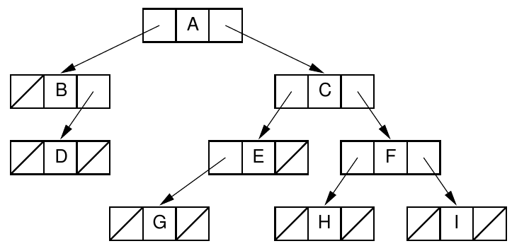
What does each node store?
Pointer based binary trees Do all nodes need to store the same
data?

Review: binary search through arrays was efficient.
Find 7:
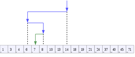
Reminder: cost of sort versus search?
What is the complexity of the operation of inserting in sorted
order,
like our sorted array list (covered before)?
Like ordered arrays, binary search trees keep their keys in sorted
order.
But, binary search trees can maintain sorted order more efficiently.
BST is a tree whose internal nodes each store a comparable or
key
(and optionally an associated value),
and each key must be greater than any key stored in its left
sub-tree,
and less than (or sometimes equal to) any key stored in its right
sub-tree.
For every node, X, in the tree,
the values of all the keys in its left subtree are smaller than the key
in X,
and the values of all the keys in its right subtree are larger than the
key in X.
Fast lookup, addition and removal of keys (\(\log_2 n\)).
On average, each lookup, insertion or deletion takes time,
proportional to the logarithm of the number of items stored in the
tree.
This is the key advantage over a continuously sorted list.
Binary search trees (BST)
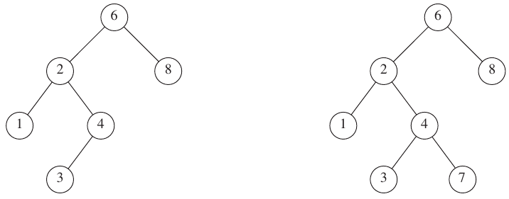
Left is a binary search tree, right is just a binary tree
Data structures
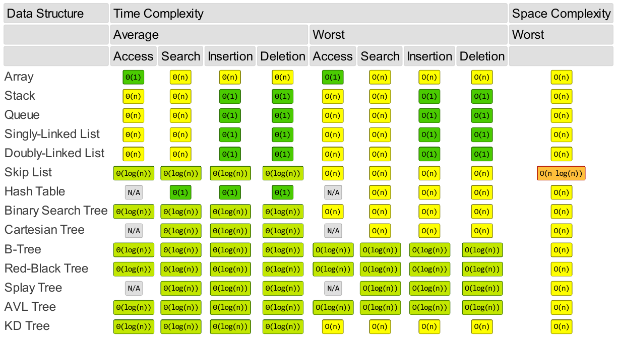
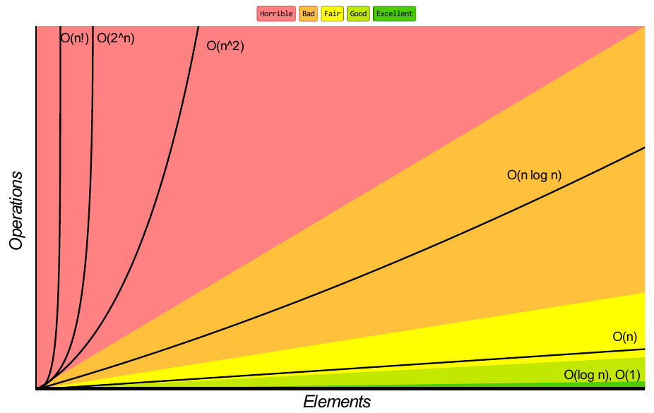
Color key:

What are steps for search?
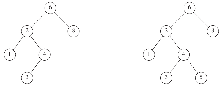
What are steps?
Delete with 0 children? Delete 35
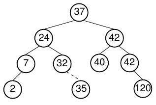
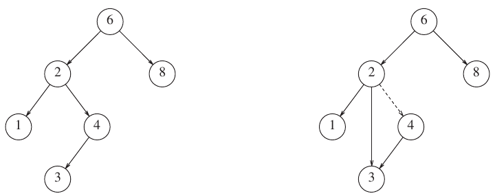
What are steps?
Delete with one child Delete 4
What are steps?
Delete with two children Delete 42, or 37, or 24?
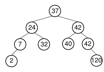
What to do with the two remaining subtrees?
Inefficient option:
Set R’s parent to point to one of R’s subtrees,
and then reinsert the remaining subtree’s nodes one at a time.
Delete with two children Delete the node labeled 2
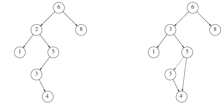
Find value in one of the subtrees that can replace the value in R.
Least key value greater than (or equal to) the one being
removed,
or else the greatest key value less than the one being removed.
Min of Max and Max of Min can be promoted to root.
Clear or delete all? For a recursive traversal that deletes all
nodes,
what order should the traversal be?

Insert order

Insert order Random tree before (left) and after (right) 250,000 insert and remove operations
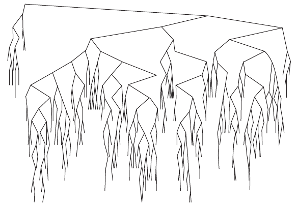
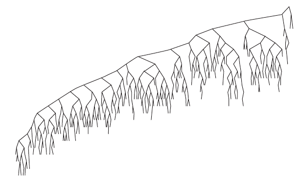
Advanced variations maintain balance during insert and remove.
The efficiency of the bstSearch algorithm is extremely sensitive to the
shape of the tree.
If the tree is perfectly balanced, the search time is log n,
but it is possible for the tree to be completely unbalanced.
This causes the bstSearch to behave much like a linear search, requiring
linear time.
We will implement an auto-balancing tree later!
With unique values, BST either implement searching for some value, k, in either:
a Map collection of pairs of (k,v) where k is
unique,
and the v is the relevant value is returned.
or a Set collection of unique k, and membership itself
is relevant.
There is an interesting point to notice about binary search
trees.
Sometimes the properties that a data structure must satisfy are specified
completely by its type.
For example, a linear search algorithm can be applied to list of
key-value pairs,
as long as the list has the right type, [(a,b)].
In contrast, the binary search tree must be of the right type,
but it must also satisfy the ordering constraint.
Many data structures are like this,
with some additional properties required beyond just the type.
The distinction is important,
because the type of the data structure can be checked by the
compiler,
whereas the additional properties cannot.
The type system of a programming language provides a way to describe
required properties,
that can be checked at compile time;
if the type checking indicates no problem,
then it is guaranteed that the program will never generate any mis-typed
data,
that lacks the necessary properties.
For example, we said above that the linear search algorithm requires its
database to have a certain type.
When the compiler checks the type of the program and finds no type
errors,
this constitutes a formal proof,
that the program will never generate a database for the linear search
which is in the wrong form,
and could thus cause a runtime error.
The type system is unable, however, to prove that:
a binary search tree built using the insert function satisfies the
required properties.
Therefore the programmer needs to do the proof manually.
In low-level programming languages,
you need to use pointers or classes in order to process a tree.
Haskell allows you to define tree structures directly,
and offers good support for writing programs that manipulate trees.
This is especially important as there is not just one kind of
tree;
it is common to define new tree types that are tailored specifically for a
particular application.
Specifying trees formally in Haskell ensures that the data structures
are expressed precisely,
and it also makes algorithms on trees executable on a computer.
-- # Software Tools for Discrete Mathematics
module Stdm05Trees where

import Test.QuickCheck

-- # Chapter 5.  Trees

data Tree a = Leaf | Node a (Tree a) (Tree a)
  deriving (Show, Eq)

-- |
-- >>> t1
-- Node 6 Leaf Leaf
t1 :: Tree Int
t1 = Node 6 Leaf Leaf

-- |
-- >>> t2
-- Node 5 (Node 3 Leaf Leaf) (Node 8 (Node 6 Leaf Leaf) (Node 12 Leaf Leaf))
t2 :: Tree Int
t2 =
  Node
    5
    (Node 3 Leaf Leaf)
    ( Node
        8
        (Node 6 Leaf Leaf)
        (Node 12 Leaf Leaf)
    )

-- |
-- >>> nodeCount t2
-- 5
nodeCount :: Tree a -> Int
nodeCount Leaf = 0
nodeCount (Node x t1 t2) = 1 + nodeCount t1 + nodeCount t2

-- |
-- >>> height t2
-- 3
height :: Tree a -> Int
height Leaf = 0
height (Node x t1 t2) = 1 + max (height t1) (height t2)

-- |
-- >>> reflect t2
-- Node 5 (Node 8 (Node 12 Leaf Leaf) (Node 6 Leaf Leaf)) (Node 3 Leaf Leaf)
reflect :: Tree a -> Tree a
reflect Leaf = Leaf
reflect (Node a t1 t2) = Node a (reflect t2) (reflect t1)

-- |
-- >>> mapTree (5 *) t2
-- Node 25 (Node 15 Leaf Leaf) (Node 40 (Node 30 Leaf Leaf) (Node 60 Leaf Leaf))
mapTree :: (a -> b) -> Tree a -> Tree b
mapTree f Leaf = Leaf
mapTree f (Node a t1 t2) = Node (f a) (mapTree f t1) (mapTree f t2)

-- | This is like a dictionary of (fst, snd)
-- >>> t3
-- Node (5,10) (Node (3,6) (Node (1,1) Leaf Leaf) (Node (4,8) Leaf Leaf)) (Node (7,14) (Node (6,12) Leaf Leaf) (Node (8,16) Leaf Leaf))
t3 :: Tree (Int, Int)
t3 =
  Node
    (5, 10)
    ( Node
        (3, 6)
        (Node (1, 1) Leaf Leaf)
        (Node (4, 8) Leaf Leaf)
    )
    ( Node
        (7, 14)
        (Node (6, 12) Leaf Leaf)
        (Node (8, 16) Leaf Leaf)
    )

-- |
-- >>> balanced t2
-- False

-- |
-- >>> balanced t3
-- True
balanced :: Tree a -> Bool
balanced Leaf = True
balanced (Node x t1 t2) = balanced t1 && balanced t2 && (height t1 == height t2)

-- |
-- >>> inorder t2
-- [3,5,6,8,12]
inorder :: Tree a -> [a]
inorder Leaf = []
inorder (Node x t1 t2) = inorder t1 ++ [x] ++ inorder t2

-- |
-- >>> preorder t2
-- [5,3,8,6,12]
preorder :: Tree a -> [a]
preorder Leaf = []
preorder (Node x t1 t2) = [x] ++ preorder t1 ++ preorder t2

-- |
-- >>> postorder t2
-- [3,6,12,8,5]
postorder :: Tree a -> [a]
postorder Leaf = []
postorder (Node x t1 t2) = postorder t1 ++ postorder t2 ++ [x]

-- | This prints nicely; show it!
-- >>> putStrLn (inorderBackwards t2 "")
-- "\n\n    \n            Leaf\n        12\n            Leaf\n    8\n    \n            Leaf\n        6\n            Leaf\n5\n\n        Leaf\n    3\n        Leaf"
inorderBackwards :: (Show a) => Tree a -> String -> String
inorderBackwards Leaf indent = "    " ++ "Leaf"
inorderBackwards (Node x t1 t2) indent =
  ( "\n"
      ++ indent
      ++ inorderBackwards t2 (indent ++ "    ")
      ++ "\n"
      ++ indent
      ++ show x
      ++ "\n"
      ++ indent
      ++ inorderBackwards t1 (indent ++ "    ")
  )

-- Expression trees

data Exp
  = Const Int
  | Add Exp Exp
  | Mult Exp Exp
  deriving (Show, Eq)

-- |
-- >>> t4
-- Mult (Const 2) (Add (Const 5) (Const 3))
t4 :: Exp
t4 = Mult (Const 2) (Add (Const 5) (Const 3))

-- | (*) 2 ((+) 5 3)
-- >>> eval t4
-- 16
eval :: Exp -> Int
eval (Const n) = n
eval (Add e1 e2) = eval e1 + eval e2
eval (Mult e1 e2) = eval e1 * eval e2

-- Binary Search Trees are ordered left to right, and must remain ordered!
-- They are more efficient than search through lists, like this:

-- | This searches through a list of (fst, snd) for fst, and returns snd.
-- >>> linSearch 11 (zip [1..] ['a'..'z'])
-- Just 'k'
linSearch :: (Eq a) => a -> [(a, b)] -> Maybe b
linSearch k [] = Nothing
linSearch k ((x, y) : xs) =
  if k == x
    then Just y
    else linSearch k xs

-- Tree t3 tree is ordered. See:
-- putStrLn (inorderBackwards t3 "")

-- | This searches through a tree of (fst, snd) for fst, and returns snd.
-- >>> bstSearch 7 t3
-- Just 14
bstSearch :: (Ord a) => a -> Tree (a, b) -> Maybe b
bstSearch key Leaf = Nothing
bstSearch key (Node (x, y) t1 t2) =
  if key == x
    then Just y
    else
      if key < x
        then bstSearch key t1
        else bstSearch key t2

-- | This function preserves the ordering of the BST!
-- >>> insertTree (2,5) t3
-- Node (5,10) (Node (3,6) (Node (1,1) Leaf (Node (2,5) Leaf Leaf)) (Node (4,8) Leaf Leaf)) (Node (7,14) (Node (6,12) Leaf Leaf) (Node (8,16) Leaf Leaf))
insertTree :: (Ord a) => (a, b) -> Tree (a, b) -> Tree (a, b)
insertTree (key, d) Leaf = Node (key, d) Leaf Leaf
insertTree (key, d) (Node (x, y) t1 t2) =
  if key == x
    then Node (key, d) t1 t2
    else
      if key < x
        then Node (x, y) (insertTree (key, d) t1) t2
        else Node (x, y) t1 (insertTree (key, d) t2)

-- Tree t3 tree is still ordered. Show this in ghci in class:
-- putStrLn (inorderBackwards (insertTree (2,5) t3) "")

-- Induction on trees

-- Theorem 29. Let t :: BinTree a.
-- Then reflect (reflect t) = t.
-- Proof. The proposition P (t) that we need to prove says reflect (reflect t) = t.
-- The theorem is proved by induction over t.

-- | The base case
-- >>> reflectBase Leaf
-- True
reflectBase :: (Eq a) => Tree a -> Bool
reflectBase t = (reflect . reflect) t == t

-- For the inductive case, let t1, t2 :: BinTree a be trees, and assume P (t1) and P (t2).
-- These are the inductive hypotheses.
-- The aim is to prove that the proposition holds for a larger tree P (Node x t1 t2).

-- | Inductive case + 1
-- >>> quickCheck reflectInductive
-- +++ OK, passed 100 tests.
reflectInductive :: (Eq a) => a -> Bool
reflectInductive val =
  let t = Node val Leaf Leaf
   in (reflect . reflect) t == t

-- Theorem 30. Let t :: BinTree a be an arbitrary binary tree of finite size.
-- Then inorder (reflect t) = reverse (inorder t).

-- | Base case
-- >>> reverseBase Leaf
-- True
reverseBase :: (Eq a) => Tree a -> Bool
reverseBase t = inorder (reflect t) == reverse (inorder t)

-- | Inductive case + 1
-- >>> quickCheck reverseInductive
-- +++ OK, passed 100 tests.
reverseInductive :: (Eq a) => a -> Bool
reverseInductive val =
  let t = Node val Leaf Leaf
   in inorder (reflect t) == reverse (inorder t)

-- Theorem 31. Let h = height t. If balanced t, then size t = 2h − 1.
-- Proof. The proposition we want to prove is: balanced t → size t = 2h − 1.
-- The proof is an induction over the tree structure.
-- For the base case, we need to prove that the theorem holds for a leaf.

-- | Base case
-- >>> sizeHeightBase Leaf
-- True
sizeHeightBase :: (Eq a) => Tree a -> Bool
sizeHeightBase t =
  if balanced t
    then nodeCount t == (2 ^ (height t)) - 1
    else error "Starting assumption not met"

-- | Inductive case + 1
-- >>> quickCheck sizeHeightInductive
-- +++ OK, passed 100 tests.
sizeHeightInductive :: (Eq a) => a -> Bool
sizeHeightInductive val =
  let t = Node val Leaf Leaf
   in if balanced t
        then nodeCount t == (2 ^ (height t)) - 1
        else error "Starting assumption not met"

-- Theorem 32. Let t :: BinTree a be any finite binary tree. Then length (inorder t) = size t.

-- | Base case
-- >>> flatLengthBase Leaf
-- True
flatLengthBase :: (Eq a) => Tree a -> Bool
flatLengthBase t = length (inorder t) == nodeCount t

-- | Inductive case + 1
-- >>> quickCheck flatLengthInductive
-- +++ OK, passed 100 tests.
flatLengthInductive :: (Eq a) => a -> Bool
flatLengthInductive val =
  let t = Node val Leaf Leaf
in length (inorder t) == nodeCount tmodule HL07IAR where
import Data.List
import HL04STAL (display)
-- Sum of first n odd numbers
-- |
-- >>> sumOddsManual 42
-- 1764
sumOddsManual :: Int -> Integer
sumOddsManual n = sum (take n [1, 3 ..])
-- |
-- >>> sumOdds' 42
-- 1764
sumOdds' :: Integer -> Integer
sumOdds' n = sum [2 * k - 1 | k <- [1 .. n]]
-- |
-- >>> sumOdds 42
-- 1764
sumOdds :: Integer -> Integer
sumOdds n = n ^ 2
-- Sum of of first n evens
-- |
-- >>> sumEvensManual 42
-- 1806
sumEvensManual :: Int -> Integer
sumEvensManual n = sum (take n [2, 4 ..])
-- |
-- >>> sumEvens' 42
-- 1806
sumEvens' :: Integer -> Integer
sumEvens' n = sum [2 * k | k <- [1 .. n]]
-- |
-- >>> sumEvens' 42
-- 1806
sumEvens :: Integer -> Integer
sumEvens n = n * (n + 1)
-- Just divide that by 2!
-- Sum of of first n ints
-- |
-- >>> sumIntsManual 42
-- 903
sumIntsManual :: Int -> Integer
sumIntsManual n = sum (take n [1, 2 ..])
-- |
-- >>> sumInts 42
-- 903
sumInts :: Integer -> Integer
sumInts n = div (n * (n + 1)) 2
-- Sum of of first n squares
-- |
-- >>> sumSquares' 42
-- 25585
sumSquares' :: Integer -> Integer
sumSquares' n = sum [k ^ 2 | k <- [1 .. n]]
-- |
-- >>> sumSquares 42
-- 25585
sumSquares :: Integer -> Integer
sumSquares n = div (n * (n + 1) * (2 * n + 1)) 6
-- Sum of of first n cubes
-- |
-- >>> sumCubes' 42
-- 815409
sumCubes' :: Integer -> Integer
sumCubes' n = sum [k ^ 3 | k <- [1 .. n]]
-- |
-- >>> sumCubes 42
-- 815409
sumCubes :: Integer -> Integer
sumCubes n = div (n * (n + 1)) 2 ^ 2
-- Another implementation of Peano arithmitic
-- Z is Zero
-- S is Successor
data Natural = Z | S Natural
deriving (Eq, Show)
-- | 1 + 2
-- >>> plus (S Z) (S (S Z))
-- S (S (S Z))
plus m Z = m
plus m (S n) = S (plus m n)
-- | 2 * 2
-- >>> mult (S (S Z)) (S (S Z))
-- S (S (S (S Z)))
mult m Z = Z
mult m (S n) = plus (mult m n) m
-- | 2^3
-- >>> expn (S (S Z)) (S (S (S Z)))
-- S (S (S (S (S (S (S (S Z)))))))
expn m Z = S Z
expn m (S n) = mult (expn m n) m
-- | 2 <= 3
-- >>> leq (S (S Z)) (S (S (S Z)))
-- True
leq Z _ = True
leq (S _) Z = False
leq (S m) (S n) = leq m n
-- | 2 >= 3
-- >>> geq (S (S Z)) (S (S (S Z)))
-- False
geq m n = leq n m
-- | 2 > 3
-- >>> geq (S (S Z)) (S (S (S Z)))
-- False
gt m n = not (leq m n)
-- | 2 < 3
-- >>> leq (S (S Z)) (S (S (S Z)))
-- True
lt m n = gt n m
-- | 7.14
-- >>> subtr (S (S Z)) (S Z)
-- S Z
subtr :: Natural -> Natural -> Natural
subtr Z _ = Z
subtr m Z = m
subtr (S m) (S n) = subtr m n
-- | 7.15
-- >>> qrm (S (S (S Z))) (S (S Z))
-- (S Z,S Z)
qrm :: Natural -> Natural -> (Natural, Natural)
qrm m n
| gt n m = (Z, m)
| otherwise = (S (fst qr), snd qr)
where
qr = qrm (subtr m n) n
-- |
-- >>> quotient (S (S (S Z))) (S (S Z))
-- S Z
quotient :: Natural -> Natural -> Natural
quotient m n = fst (qrm m n)
-- |
-- >>> remainder (S (S (S Z))) (S (S Z))
-- S Z
remainder :: Natural -> Natural -> Natural
remainder m n = snd (qrm m n)
-- This enables a generalized re-write of the above functions:
foldn :: (a -> a) -> a -> Natural -> a
foldn h c Z = c
foldn h c (S n) = h (foldn h c n)
-- | 1 + 2
-- >>> plus' (S Z) (S (S Z))
-- S (S (S Z))
plus' :: Natural -> Natural -> Natural
plus' = foldn (\n -> S n)
-- | 2 * 2
-- >>> mult' (S (S Z)) (S (S Z))
-- S (S (S (S Z)))
mult' :: Natural -> Natural -> Natural
mult' m = foldn (plus' m) Z
-- | 2^3
-- >>> expn' (S (S Z)) (S (S (S Z)))
-- S (S (S (S (S (S (S (S Z)))))))
expn' :: Natural -> Natural -> Natural
expn' m = foldn (mult' m) (S Z)
-- | 7.16
-- >>> subtr2 (S (S Z)) (S Z)
-- S Z
pre :: Natural -> Natural
pre Z = Z
pre (S n) = n
subtr2 :: Natural -> Natural -> Natural
subtr2 = foldn pre
-- |
-- >>> exclaim (S (S Z))
-- "!!"
exclaim :: Natural -> String
exclaim = foldn ('!' :) []
-- Selects bitlists without consecutive zeros.
bittest :: [Int] -> Bool
bittest [] = True
bittest [0] = True
bittest (1 : xs) = bittest xs
bittest (0 : 1 : xs) = bittest xs
bittest _ = False
fib 0 = 0
fib 1 = 1
fib n = fib (n - 1) + fib (n - 2)
fib' n = fib2 0 1 n
where
fib2 a b 0 = a
fib2 a b n = fib2 b (a + b) (n - 1)
-- | 7.20 Write a function that generates: https://en.wikipedia.org/wiki/Catalan_number
-- >>> catalan 6
-- 132
catalan :: Integer -> Integer
catalan 0 = 1
catalan n = sum [catalan i * catalan ((n - 1) - i) | i <- [0 .. (n - 1)]]
-- Trees
data BinTree = L | N BinTree BinTree
deriving (Show)
-- |
-- >>> makeBinTree 2
-- N (N L L) (N L L)
makeBinTree :: Integer -> BinTree
makeBinTree 0 = L
makeBinTree n = N (makeBinTree (n - 1)) (makeBinTree (n - 1))
-- |
-- >>> count (makeBinTree 2)
-- 7
count :: BinTree -> Integer
count L = 1
count (N t1 t2) = 1 + count t1 + count t2
-- |
-- >>> depth (makeBinTree 2)
-- 2
depth :: BinTree -> Integer
depth L = 0
depth (N t1 t2) = max (depth t1) (depth t2) + 1
-- |
-- >>> balanced (makeBinTree 2)
-- True
balanced :: BinTree -> Bool
balanced L = True
balanced (N t1 t2) =
balanced t1
&& balanced t2
&& depth t1 == depth t2
-- 7.25 Write a Haskell definition of ternary trees, plus procedures for generating balanced ternary trees and counting their node numbers.
data TernTree = L' | N' TernTree TernTree TernTree
deriving (Show)
-- |
-- >>> makeTernTree 2
-- N' (N' L' L' L') (N' L' L' L') (N' L' L' L')
makeTernTree :: Integer -> TernTree
makeTernTree 0 = L'
makeTernTree n = N' (makeTernTree (n - 1)) (makeTernTree (n - 1)) (makeTernTree (n - 1))
-- |
-- >>> count3 (makeTernTree 2)
-- 13
count3 :: TernTree -> Integer
count3 L' = 1
count3 (N' t1 t2 t3) = 1 + count3 t1 + count3 t2 + count3 t3
-- | A binary tree container Int data
-- >>> Nd 5 (Nd 2 Lf Lf) (Nd 3 Lf Lf)
-- Nd 5 (Nd 2 Lf Lf) (Nd 3 Lf Lf)
data Tree = Lf | Nd Int Tree Tree
deriving (Show)
-- | 7.28 Write a function that inserts a number n in an ordered tree in such a way that the tree remains ordered.
-- >>> insertTree 4 (Nd 5 (Nd 2 Lf Lf) (Nd 3 Lf Lf))
-- Nd 5 (Nd 2 Lf (Nd 4 Lf Lf)) (Nd 3 Lf Lf)
insertTree :: Int -> Tree -> Tree
insertTree n Lf = Nd n Lf Lf
insertTree n t@(Nd m left right)
| m < n = Nd m left (insertTree n right)
| m > n = Nd m (insertTree n left) right
| otherwise = t
-- | 7.29
-- >>> list2tree [1..5]
-- Nd 5 (Nd 4 (Nd 3 (Nd 2 (Nd 1 Lf Lf) Lf) Lf) Lf) Lf
list2tree :: [Int] -> Tree
list2tree [] = Lf
list2tree (n : ns) = insertTree n (list2tree ns)
-- |
-- >>> tree2list (list2tree [1..5])
-- [1,2,3,4,5]
tree2list :: Tree -> [Int]
tree2list Lf = []
tree2list (Nd n left right) = tree2list left ++ [n] ++ tree2list right
-- | 7.30 Write a function that checks whether a given integer i occurs in an ordered tree.
-- >>> inTree 7 (Nd 5 (Nd 2 Lf Lf) (Nd 7 Lf Lf))
-- True
inTree :: Int -> Tree -> Bool
inTree n Lf = False
inTree n (Nd m left right)
| n == m = True
| n < m = inTree n left
| n > m = inTree n right
-- | 7.31 Merges two trees, produces ordered tree.
-- >>> mergeTrees (Nd 5 (Nd 2 Lf Lf) (Nd 7 Lf Lf)) (Nd 6 (Nd 1 Lf Lf) (Nd 8 Lf Lf))
-- Nd 6 (Nd 1 Lf (Nd 5 (Nd 2 Lf Lf) Lf)) (Nd 8 (Nd 7 Lf Lf) Lf)
mergeTrees :: Tree -> Tree -> Tree
mergeTrees t1 t2 = foldr insertTree t2 (tree2list t1)
-- | 7.32 Finds depth of a given element
-- >>> findDepth 7 (Nd 5 (Nd 2 Lf Lf) (Nd 7 Lf Lf))
-- 1
findDepth :: Int -> Tree -> Int
findDepth _ Lf = -1
findDepth n (Nd m left right)
| n == m = 0
| n < m = if d1 == -1 then -1 else d1 + 1
| n > m = if d2 == -1 then -1 else d2 + 1
where
d1 = findDepth n left
d2 = findDepth n right
-- | A binary tree container for any data, a
-- >>> T 5 (T 2 Nil Nil) (T 3 Nil Nil)
-- T 5 (T 2 Nil Nil) (T 3 Nil Nil)
data Tr a = Nil | T a (Tr a) (Tr a)
deriving (Eq, Show)
-- | 7.33 Like map, but for trees
-- >>> mapT (1 +) (T 5 (T 2 Nil Nil) (T 3 Nil Nil))
-- T 6 (T 3 Nil Nil) (T 4 Nil Nil)
mapT :: (a -> b) -> Tr a -> Tr b
mapT f Nil = Nil
mapT f (T x left right) = T (f x) (mapT f left) (mapT f right)
-- | 7.34 Like fold, but for trees
-- >>> foldT (\x y z -> x + y + z) 0 (T 5 (T 2 Nil Nil) (T 3 Nil Nil))
-- 10
foldT :: (a -> b -> b -> b) -> b -> Tr a -> b
foldT h c Nil = c
foldT h c (T x left right) = h x (foldT h c left) (foldT h c right)
-- 7.35 traversals using fold
-- |
-- >>> preorderT (T 5 (T 2 Nil Nil) (T 3 Nil Nil))
-- [5,2,3]
preorderT :: Tr a -> [a]
preorderT = foldT preLists []
where
preLists x ys zs = (x : ys) ++ zs
-- |
-- >>> inorderT (T 5 (T 2 Nil Nil) (T 3 Nil Nil))
-- [2,5,3]
inorderT :: Tr a -> [a]
inorderT = foldT inLists []
where
inLists x ys zs = ys ++ [x] ++ zs
-- |
-- >>> postorderT (T 5 (T 2 Nil Nil) (T 3 Nil Nil))
-- [2,3,5]
postorderT :: Tr a -> [a]
postorderT = foldT postLists []
where
postLists x ys zs = ys ++ zs ++ [x]
-- 7.36 Checks if tree is ordered
-- |
-- >>> orderedT (T 5 (T 2 Nil Nil) (T 3 Nil Nil))
-- False
-- |
-- >>> orderedT (T 5 (T 2 Nil Nil) (T 8 Nil Nil))
-- True
orderedT :: (Ord a) => Tr a -> Bool
orderedT tree = ordered (inorderT tree)
where
ordered xs = sort (nub xs) == xs
-- A dictionary example:
type Dict = Tr (String, String)
-- | 7.37
-- >>>
lookupD :: String -> Dict -> [String]
lookupD _ Nil = []
lookupD x (T (v, w) left right)
| x == v = [w]
| x < v = lookupD x left
| otherwise = lookupD x right
split :: [a] -> ([a], a, [a])
split xs = (ys1, y, ys2)
where
ys1 = take n xs
(y : ys2) = drop n xs
n = length xs `div` 2
data LeafTree a
= Leaf a
| Node (LeafTree a) (LeafTree a)
deriving (Show)
ltree :: LeafTree String
ltree =
Node
(Leaf "I")
( Node
(Leaf "love")
(Leaf "you")
)
data Rose a = Bud a | Br [Rose a]
deriving (Eq, Show)
rose = Br [Bud 1, Br [Bud 2, Bud 3, Br [Bud 4, Bud 5, Bud 6]]]
len [] = 0
len (x : xs) = 1 + len xs
cat :: [a] -> [a] -> [a]
cat [] ys = ys
cat (x : xs) ys = x : cat xs ys
add :: [Natural] -> Natural
add = foldr plus Z
mlt :: [Natural] -> Natural
mlt = foldr mult (S Z)
ln :: [a] -> Natural
ln = foldr (\_ n -> S n) Z
rev :: [a] -> [a]
rev = foldl (\xs x -> x : xs) []
rev' :: [a] -> [a]
rev' = foldr (\x xs -> xs ++ [x]) []
data Peg = A | B | C
type Tower = ([Int], [Int], [Int])
move :: Peg -> Peg -> Tower -> Tower
move A B (x : xs, ys, zs) = (xs, x : ys, zs)
move B A (xs, y : ys, zs) = (y : xs, ys, zs)
move A C (x : xs, ys, zs) = (xs, ys, x : zs)
move C A (xs, ys, z : zs) = (z : xs, ys, zs)
move B C (xs, y : ys, zs) = (xs, ys, y : zs)
move C B (xs, ys, z : zs) = (xs, z : ys, zs)
transfer :: Peg -> Peg -> Peg -> Int -> Tower -> [Tower]
transfer _ _ _ 0 tower = [tower]
transfer p q r n tower =
transfer p r q (n - 1) tower
++ transfer r q p (n - 1) (move p q tower')
where
tower' = last (transfer p r q (n - 1) tower)
hanoi :: Int -> [Tower]
hanoi n = transfer A C B n ([1 .. n], [], [])
check :: Int -> Tower -> Bool
check 0 t = t == ([], [], [])
check n (xs, ys, zs)
| xs /= [] && last xs == n = check (n - 1) (init xs, zs, ys)
| zs /= [] && last zs == n = check (n - 1) (ys, xs, init zs)
| otherwise = False
maxT :: Tower -> Int
maxT (xs, ys, zs) = foldr max 0 (xs ++ ys ++ zs)
checkT :: Tower -> Bool
checkT t = check (maxT t) t
parity :: Tower -> (Int, Int, Int)
parity (xs, ys, zs) = par (xs ++ [n + 1], ys ++ [n], zs ++ [n + 1])
where
n = maxT (xs, ys, zs)
par (x : xs, y : ys, z : zs) = (mod x 2, mod y 2, mod z 2)
target :: Tower -> Peg
target t@(xs, ys, zs)
| parity t == (0, 1, 1) = A
| parity t == (1, 0, 1) = B
| parity t == (1, 1, 0) = C
move1 :: Tower -> Tower
move1 t@(1 : _, ys, zs) = move A (target t) t
move1 t@(xs, 1 : _, zs) = move B (target t) t
move1 t@(xs, ys, 1 : _) = move C (target t) t
move2 :: Tower -> Tower
move2 t@(1 : xs, [], zs) = move C B t
move2 t@(1 : xs, ys, []) = move B C t
move2 t@(1 : xs, ys, zs) = if ys < zs then move B C t else move C B t
move2 t@([], 1 : ys, zs) = move C A t
move2 t@(xs, 1 : ys, []) = move A C t
move2 t@(xs, 1 : ys, zs) = if xs < zs then move A C t else move C A t
move2 t@([], ys, 1 : zs) = move B A t
move2 t@(xs, [], 1 : zs) = move A B t
move2 t@(xs, ys, 1 : zs) = if xs < ys then move A B t else move B A t
done :: Tower -> Bool
done ([], [], _) = True
done (xs, ys, zs) = False
transfer1, transfer2 :: Tower -> [Tower]
transfer1 t = t : transfer2 (move1 t)
transfer2 t = if done t then [t] else t : transfer1 (move2 t)
hanoi' :: Int -> [Tower]
hanoi' n = transfer1 ([1 .. n], [], [])
zazen :: [Tower]
zazen = hanoi' 64
hanoiCount :: Int -> Integer -> Tower
hanoiCount n k
| k < 0 = error "argument negative"
| k > 2 ^ n - 1 = error "argument not in range"
| k == 0 = ([1 .. n], [], [])
| k == 2 ^ n - 1 = ([], [], [1 .. n])
| k < 2 ^ (n - 1) = (xs ++ [n], zs, ys)
| k >= 2 ^ (n - 1) = (ys', xs', zs' ++ [n])
where
(xs, ys, zs) = hanoiCount (n - 1) k
(xs', ys', zs') = hanoiCount (n - 1) (k - 2 ^ (n - 1))
toTower :: Integer -> Tower
toTower n = hanoiCount k m
where
n' = fromInteger (n + 1)
k = truncate (logBase 2 n')
m = truncate (n' - 2 ^ k)
data Form = P Int | Conj Form Form | Disj Form Form | Neg Form
instance Show Form where
show (P i) = 'P' : show i
show (Conj f1 f2) = "(" ++ show f1 ++ " & " ++ show f2 ++ ")"
show (Disj f1 f2) = "(" ++ show f1 ++ " v " ++ show f2 ++ ")"
show (Neg f) = "~" ++ show f
subforms :: Form -> [Form]
subforms (P n) = [P n]
subforms (Conj f1 f2) = Conj f1 f2 : (subforms f1 ++ subforms f2)
subforms (Disj f1 f2) = Disj f1 f2 : (subforms f1 ++ subforms f2)
subforms (Neg f) = Neg f : subforms f
ccount :: Form -> Int
ccount (P n) = 0
ccount (Conj f1 f2) = 1 + ccount f1 + ccount f2
ccount (Disj f1 f2) = 1 + ccount f1 + ccount f2
ccount (Neg f) = 1 + ccount f
acount :: Form -> Int
acount (P n) = 1
acount (Conj f1 f2) = acount f1 + acount f2
acount (Disj f1 f2) = acount f1 + acount f2
acount (Neg f) = acount fmodule Sol7 where
import Data.List
import HL07IAR
-- | 7.38
-- >>>
buildTree :: [a] -> Tr a
buildTree [] = Nil
buildTree xs = T m (buildTree left) (buildTree right)
where
(left, m, right) = split xs
-- | 7.39
-- >>>
mapLT :: (a -> b) -> LeafTree a -> LeafTree b
mapLT f (Leaf x) = Leaf (f x)
mapLT f (Node left right) = Node (mapLT f left) (mapLT f right)
-- | 7.40
-- >>>
reflect :: LeafTree a -> LeafTree a
reflect (Leaf x) = Leaf x
reflect (Node left right) = Node (reflect right) (reflect left)
-- | 7.42
-- >>>
mapR :: (a -> b) -> Rose a -> Rose b
mapR f (Bud x) = Bud (f x)
mapR f (Br roses) = Br (map (mapR f) roses)
-- | 7.46
-- >>>
genUnion :: (Eq a) => [[a]] -> [a]
genUnion = foldr union []
genIntersect :: (Eq a) => [[a]] -> [a]
genIntersect = foldr1 intersect
-- | 7.47
-- >>>
insrt :: (Ord a) => a -> [a] -> [a]
insrt x [] = [x]
insrt x (y : ys) = if x <= y then x : y : ys else y : insrt x ys
srt :: (Ord a) => [a] -> [a]
srt = foldr insrt []
-- | 7.51
-- >>>
ln' :: [a] -> Natural
ln' = foldl (\n _ -> S n) Z
-- Skipped questions about Tower of HanoiThere are many useful theorems about the properties of trees,
and the behaviour of functions on trees.
To prove them, we can use induction,
but the principle of induction needs to be made slightly more general
for tree structures.
The general idea behind tree induction is similar to list
induction.
The base case is used for empty trees (or leaves),
and the induction case is used for nodes.
The principle of tree induction is stated below for binary trees,
but it can be generalised to other types of tree as well.
Theorem 28 (Principle of induction on binary trees).
Let BinTree a be a binary tree type as defined above,
and let P (t) be a proposition on trees.
Suppose the following two requirements hold:
Base case:
P (BinLeaf)
Induction case:
For all t1 and t2 of type BinTree a, and all x :: a,
suppose that the proposition holds for a tree consisting of a
node,
the value a, and the subtrees t1 and t2,
provided that the proposition holds for t1 and t2.
Using the notation of the chapter on propositional logic,
this can be written formally as
P (t1) ∧ P (t2) → P (BinNode x t1 t2).
Then ∀ t :: BinTree a | P (t);
thus the proposition holds for all trees of finite size.
Carrying out a proof using tree induction is generally no harder than
list induction.
A number of examples are given below.
In all cases, we will use trees of type BinTree a, for an arbitrary type
a.
https://en.wikipedia.org/wiki/Huffman_coding
https://www.youtube.com/watch?v=JsTptu56GM8
https://www.youtube.com/watch?v=M5c_RFKVkko&t=0s
https://www.youtube.com/watch?v=umTbivyJoiI&t=33s
https://www.youtube.com/watch?v=B3y0RsVCyrw
Example frequency data:
Character Frequency Probabilities Code
A         9         0.416667      00
R         4         0.166667      01
B         4         0.166667      100
C         2         0.083333      101
D         2         0.083333      110
SP        1         0.041667      1110
.         1         0.041667      1111
The matching tree:
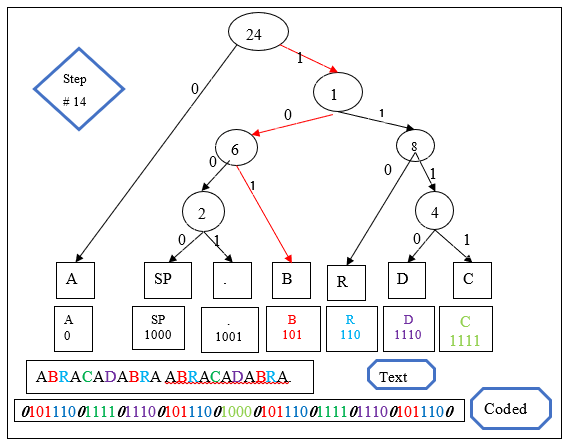
The encoding process involves a travelsal of the tree to a unique
end-point,
Thus, a bit string representing a symbol is never a prefix of
another,
which enables unambiguous parsing of this encoding.
Building the tree is a recursive process.
Encoding (compressing) text using the tree is also a recursive
tree-traversal process.
Decoding (decompressing) a code into text is also a recursive
tree-traversal process.
An accessible implementation:
Trees/Huffman.hs
#!/usr/bin/runghc

type Symbol = Char

type Weight = Float

data Node
  = Leaf Symbol Weight
  | Interior Node Node [Symbol] Weight
  deriving (Show)

getSymbols :: Node -> [Symbol]
getSymbols (Leaf s _) = [s]
getSymbols (Interior _ _ syms _) = syms

getWeight :: Node -> Weight
getWeight (Leaf _ w) = w
getWeight (Interior _ _ _ w) = w

orderedInsert :: Node -> [Node] -> [Node]
orderedInsert n [] = [n]
orderedInsert n all@(first : rest)
  | getWeight n <= getWeight first = n : all
  | otherwise = first : orderedInsert n rest

makeTree :: [Node] -> Node
makeTree [n] = n
makeTree (first : second : rest) =
  let n =
        Interior
          first
          second
          (getSymbols first ++ getSymbols second)
          (getWeight first + getWeight second)
   in makeTree (orderedInsert n rest)

-- These are derived from a large standard corpus of text.
commonTree =
  makeTree
    [ Leaf ' ' 30.2,
      Leaf 'e' 12.702,
      Leaf 't' 9.056,
      Leaf 'a' 8.167,
      Leaf 'o' 7.507,
      Leaf 'i' 6.966,
      Leaf 'n' 6.749,
      Leaf 's' 6.327,
      Leaf 'h' 6.094,
      Leaf 'r' 5.987,
      Leaf 'd' 4.253,
      Leaf 'l' 4.025,
      Leaf 'c' 2.782,
      Leaf 'u' 2.758,
      Leaf 'm' 2.406,
      Leaf 'w' 2.360,
      Leaf 'f' 2.228,
      Leaf 'g' 2.015,
      Leaf 'y' 1.974,
      Leaf 'p' 1.929,
      Leaf 'b' 1.492,
      Leaf 'v' 0.978,
      Leaf 'k' 0.772,
      Leaf 'j' 0.153,
      Leaf 'x' 0.150,
      Leaf 'q' 0.095,
      Leaf 'z' 0.071
    ]

encodeRec :: Node -> [Symbol] -> [Bool]
encodeRec _ [] = []
encodeRec (Leaf s w) (sym : symbols) = encodeRec commonTree symbols
encodeRec (Interior l r _ _) (sym : symbols)
  | elem sym (getSymbols l) = False : encodeRec l (sym : symbols)
  | otherwise = True : encodeRec r (sym : symbols)

encode = encodeRec commonTree

decodeRec :: Node -> [Bool] -> [Symbol]
decodeRec (Leaf s w) bits = s : decodeRec commonTree bits
decodeRec (Interior l _ _ _) (False : bits) = decodeRec l bits
decodeRec (Interior _ r _ _) (True : bits) = decodeRec r bits
decodeRec _ [] = []

decode = decodeRec commonTree

main :: IO ()
main = do
  putStrLn ("This is a generalized tree:\n" ++ show commonTree)

  let message = "this is a small message"
  putStrLn ("\nMessage before encoding was:\n" ++ message)
  putStrLn ("\nLength of message before encoding, times 8 was:\n" ++ show (8 * length message))

  let encoded = encode message
  putStrLn ("\nEncoded message was:\n" ++ show encoded)
  putStrLn ("\nLength of encoded message was:\n" ++ show (length encoded))

  let decoded = decode encoded
putStrLn ("\nThe decoded message was:\n" ++ decoded)The Huffman algorithm is nearly identical to this hierarchical
clustering method:
https://en.wikipedia.org/wiki/UPGMA
https://en.wikipedia.org/wiki/Hierarchical_clustering#Agglomerative_clustering_example