Previous: 02-BioAnalogyOrigins.html
“The advantage of evolutionary algorithms includes,
its ability to address problems for which there is no human
expertise.
Even though human expertise should be used when it is needed and
available;
it often proves less adequate for automated problem-solving
routines.
Certain problems exist with expert system:
the experts may not agree, may not be qualified,
may not be self-consistent or may simply cause error.
Artificial intelligence may be applied to several difficult
problems,
requiring high computational speed,
but they cannot compete with the human intelligence,
Fogel (1995) declared, they solve problems,
but they do not solve the problem of how to solve problems.
In contrast, evolutionary computation provides a that method,
for solving the problem of how to solve problems.”
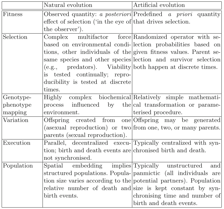
| Natural Evolution | Probleem Solving |
|---|---|
| Enivornment | Problem |
| Individual | Candidate solution |
| Fitness | Solution quality |
A population of individuals exists in an environment with limited
resources.
Competition for those resources causes differential survival
and reproduction of those fitter individuals,
that are better adapted to the particular environment they
encountered.
Fitness like the “fit of a glove”, not like “fitness of an athlete”!
These individuals act as seeds for the generation of new
individuals.
Diversity is introduced through recombination and mutation.
The new individuals have their fitness “evaluated” and “compete”
(possibly also with parents) for survival.
Over time Natural selection causes a rise in the fitness of the
population.
It causes a population’s gene pool to adapt to it’s particular past
demands.
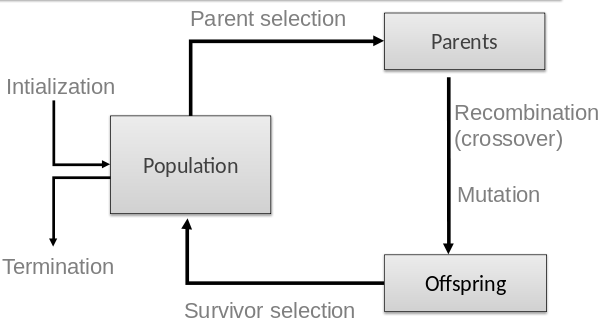
EAs fall into the category of “generate and test” algorithms.
They are stochastic, population-based algorithms.
Variation operators (recombination and mutation) create the necessary
diversity,
and thereby facilitate novelty.
Selection reduces diversity,
and acts as a force pushing or selecting for quality.
Outline for the day:
Recombination happens at a slightly different stage in living
organisms,
but it’s logically equivalent.
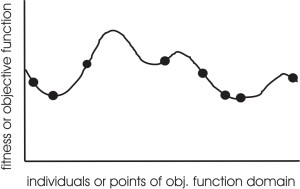
Optimization according to some fitness-criterion
(optimization on a fitness landscape)
There are two competing forces:
If these two occur with differential survival,
evolution must happen (in general)
Further, for evolution to occur (success),
we cannot ignore either.
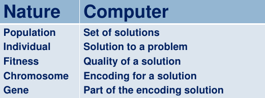
The following major parts are to be defined for each problem to be solved:
Representation
Fitness function (a.k.a. objective function)
Selection mechanisms
Initialization parameters
Parameter choices
Termination condition
Role:
Provides code for candidate solutions that can be manipulated by
variation operators.
Leads to two levels of existence:
Implies two mappings:
Chromosomes contain genes,
which are in positions called loci,
and have a value (allele):
Example representation: represent integer values by their binary
code
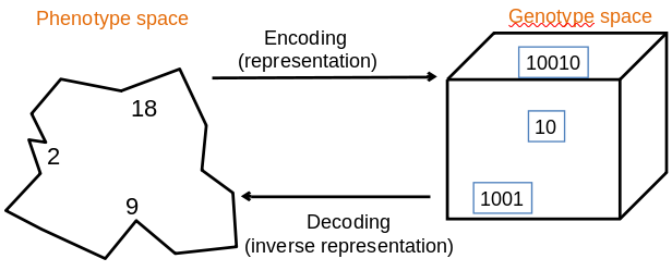
In order to find the global optimum,
every feasible solution must be represented in genotype space
A fitness function is a particular type of objective function,
that is used to summarize, as a single figure of merit,
how close a given design solution is to achieving the set aims.
Role:
Represents the task to solve, the requirements to adapt to.
Can be seen as “the environment”.
Enables selection (since it provides basis for comparison).
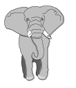
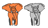
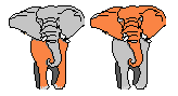
Some phenotypic traits may be advantageous, desirable,
e.g. big ears,
these traits are rewarded by more offspring that will expectedly carry
the same trait
Assigns a single real-valued fitness to each individual
phenotype.
This number forms the basis for selection.
Thus, more discrimination (large range of different values) is
better.
Typically we talk about fitness being maximized.
Some problems may be best posed as minimization problems,
but conversion is a trivial inversion.
Role:
Holds the candidate solutions of the problem as individuals
(genotypes).
Formally, a population is a multi-set of individuals,
Repetitions are possible.
Population is the basic unit of evolution,
The population is evolving, not the individuals.
Selection operators act on population level.
Variation operators act on individual level.
Selection operators usually take whole population into account.
Reproductive probabilities are relative to the current
generation.
Some sophisticated EAs also assert a spatial structure on the
population, like a grid.
Diversity of a population refers to the number of different fitnesses
/ phenotypes / genotypes present.
Each of those is not the same thing.
There are many algorithms for define diversity formally.
One can build an EC to increase mutation rates,
if diversity drops too low.
Two main types:
1. Parent selection (who gets to breed to produce children).
2. Survivor selection (which children get to live into the next
iteration, to potentially breed later)
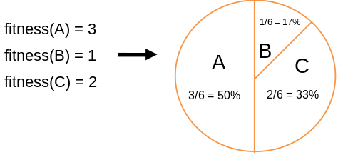
Example: roulette wheel selection
In principle,
any selection mechanism can be used for parent selection,
as well as for survivor selection
Most EAs use fixed population size,
so need a way of going from (parents + offspring) to next
generation.
Often deterministic (while parent selection is usually stochastic).
Fitness based: rank parents + new offspring, and take best.
Age based: create as many offspring as parents, and delete all/some
parents.
Sometimes a combination of stochastic and deterministic (elitism).
Proportional selection:
Parents are chosen to mate,
with probability proportional to their fitness.
Traditionally, children replace their parents,
but if best parents remain, it is called “elitism”.
Many other variations now more commonly used:
roulette wheel, tournament selection, rank-based selection,
stochastic universal sampling, truncation selection, etc.
Overall principle: survival of the fittest.
In a classical, “generational” GA:
Based on fitness, choose the set of breeders (the “intermediate”
population),
that in pairs, will be crossed over and possibly mutated,
with offspring replacing parents.
One individual may appear several times in the intermediate
population,
or the next population.
Role:
to generate new candidate solutions, with more variety.
Usually divided into two types according to their arity (number of
inputs/parents):
Arity 1 : mutation operators.
Arity >1 : recombination operators.
Arity = 2 : typically called crossover.
Arity > 2 : is formally possible, but seldom used in EC.
There has been much debate about relative importance of recombination
and mutation.
Now, most EAs use both.
Variation operators (mutation, recombination) must match the given
representation:
Tree might swap branches.
Strings might swap positions.
Numbers might randomize.
Mutation is the first type of variation operator.
Role:
Causes small, random variance.
Acts on one genotype, and delivers another.
Element of randomness is essential,
and differentiates it from other unary heuristic operators.
Importance researchers ascribe to this operation depends on
representation and historical dialect:
Binary GAs - mutation is background operator responsible for preserving
and introducing diversity.
Evolutionary programming for FSM’s / continuous variables - mutation is
the only search operator.
Genetic programming - mutation is hardly used.
May guarantee connectedness of search space,
and hence convergence proofs.
Discussion question:
Can you generate all possible solutions with enough time?
before
1 1 1 1 1 1 1
after
1 1 1 0 1 1 1

Second type of variation operator
Role:
Merges information from parents into offspring.
Choice of what information to merge is largely stochastic.
But, complements modularity in the genome.
Most offspring may be worse, or the same as the parents.
Hope is that some are better by combining elements of genotypes that
lead to good traits.
Principle has been used for millennia by breeders of plants and
livestock.
Parents
Mark middle of genome:
Parent 1: 1 1 1 | 1 1 1 1
Parent 2: 0 0 0 | 0 0 0 0
Offspring
Swap around mark to generate new genome:
Child 1: 1 1 1 | 0 0 0 0
Child 2: 0 0 0 | 1 1 1 1
Initialization is usually performed by creating a random
population.
Need to ensure even spread, and mixture of possible allele values.
Can include existing solutions, or
use problem-specific heuristics, to “seed” the population (not usually
worth the effort).
Need population size and generation size to be as large as computationally practical!
Termination condition checked every generation:
Historically different flavors of EAs have been associated with different data types to represent solutions
These differences are largely irrelevant, now the best modern
strategy is to:
Choose representation to suit your problem.
Choose variation operators to suit your representation.
Selection operators, which choose survival and reproduction,
only use abstract fitness itself,
and so are independent of the representation you choose!
Discussion question:
Recall the quote at the top of the lecture.
Does it seem like EC can solve, in part,
the problem of learning to solve problems,
that is more broad than solving the problem itself
Is this always the case,
or dependent on what you use the EC for?
We’ll go over these now:
Remember:
The following major parts are to be defined for each problem:
A trivial optimization problem:
Maximizing the value of x2 for integers,
in the range 0-31 (the full range of 5 bits).
Yes, this is a bit of a contrived example…
We’ll get to more realistic ones soon!
Must make design decisions regarding the EA components:
representation, parent selection, recombination, mutation, and survivor
selection.
The following major parts are required:
Initialize, parent selection
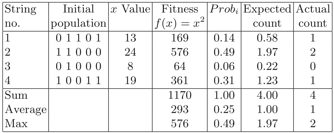
How to implement random selection in an instance?
Basic idea:
#!/usr/bin/python3

import random

rand_sample: list[int] = [1] * 14 + [2] * 49 + [3] * 6 + [4] * 31
new_pop: list[int] = []
for i in range(4):
    new_pop.append(random.choice(rand_sample))
Random magic:
#!/usr/bin/python3

import random

rand_sample: list[int] = [1, 2, 3, 4]
weights: list[float] = [0.06, 0.14, 0.31, 0.49]
new_pop: list[int] = []
new_pop = random.choices(rand_sample, weights, k=4)
Hack to do this manually, numerically, more efficiently:
#!/usr/bin/python3

new_pop: list[int] = []

for i in range(4):
    rand_sample = random.random()  # [0, 1)
    # Cumulative probabilities:
    if rand_sample < 0.06:
        new_pop.append(3)
    elif rand_sample < (0.06 + 0.14):
        new_pop.append(1)
    elif rand_sample < (0.06 + 0.14 + 0.31):
        new_pop.append(1)
    elif rand_sample < (0.06 + 0.14 + 0.31 + 0.49):  # aka < 1
        new_pop.append(2)
    # last elif could just be else...
    # but this is explicit for readability.
Cross over
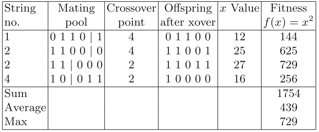
Mutation
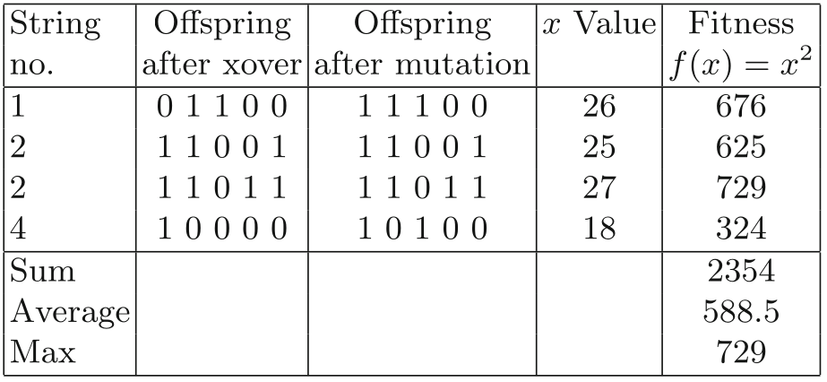
(note a couple math errors in this one…)
In this case,
the mutations shown happen to have caused positive changes in
fitness,
but we should emphasize that in later generations,
as the number of 1’s in the population rises,
mutation will be on average (but not always) deleterious.
Survival selection
Children only, no parents.
Check termination condition,
Rinse, repeat…
Code for x-squared optimization:
03-MetaheuristicParts/01_xsquared.py
https://en.wikipedia.org/wiki/Eight_queens_puzzle
Place 8 queens on an 8x8 chessboard in such a way that they cannot check
each other.
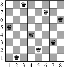
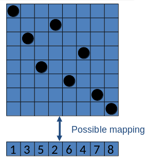
What kind of data structure do we employ,
to represent a complete solution to the n-queens problem?
Phenotype: a board configuration
Genotype: a permutation of the numbers 1-8
Penalty of one queen/gene:
the number of queens she can check.
Penalty of a whole individual/configuration/solution:
the sum of penalties of all queens.
Penalty is to be minimized.
Fitness of a configuration:
inverse penalty to be maximized.
Small variation in one permutation, e.g.:
swapping values of two randomly chosen positions
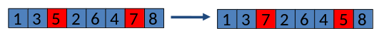
Discuss:
Why swapping instead of random single point mutation?
There are a variety of recombination options.
What is a permutation?
What is a set?
Our recombination should combine two permutations into two new
permutations.
What happens if we just pick a position,
and swap the arms, like we did with x-squared above?
Instead, we choose a random crossover point.
Copy first parts into children (somewhat like before).
Create second part by inserting values from other parent (new option
here).
in the order they appear there,
beginning after crossover point,
skipping values already in child.
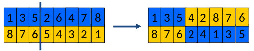
The 2nd half is a subtle operation.
Make sure you understand it!
Important discussion:
Why permutation by the opposing strand?
Does it accomplish something similar to just swapping “arms”?
Does it still capitalize on modularity?
Can you think of any other ways to recombine a permutation?
Parent selection (who breeds):
Pick 5 parents and take best two to undergo crossover.
Survivor selection (who gets replaced):
When inserting a new child into the population,
choose an existing member to replace by:
sorting the whole population by decreasing fitness,
enumerating this list from high to low, and
replacing the first with a fitness lower than the given child.
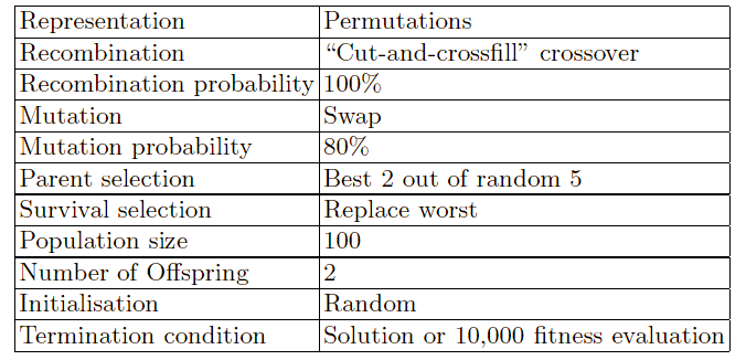
This configuration of an EC implementation is only one
possible.
There are other sets of choices of operators and parameters.
Discussion questions:
What about when there is one fewer queen…?
Example: The 7-queens problem
Can you think of any other way we could have encoded solutions to
this problem?
Would you guess those methods have been easier or harder to solve?
Code for n-queens:
03-MetaheuristicParts/02_nqueens.py
https://en.wikipedia.org/wiki/Knapsack_problem
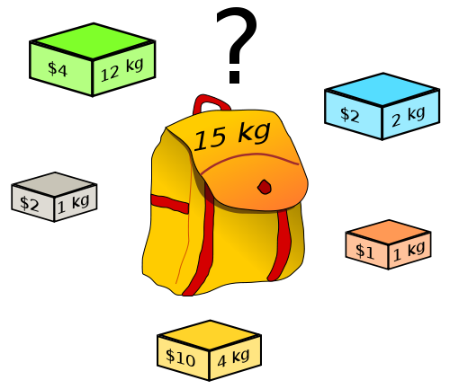
Given a set of items, each with a weight and a value,
determine the number of each item to include in a collection,
so that the total weight is less than or equal to a given limit,
and the total value is as large as possible.
There are a variety of types of knapsack problem.
The most common type being solved is the 0-1 knapsack problem,
which restricts the number xi of copies of each kind of item
to zero or one.
You are given a set of n items numbered from 1 up to n,
each with a weight wi and a value vi,
along with a maximum weight capacity W.
The task is to select a subset of those items,
that maximizes the sum of the values,
while keeping the summed cost within some capacity.
Maximize:
\(\sum_{i=1}^n v_i x_i\)
Subject to:
\(\sum_{i=1}^n w_i x_i \leq W and\ x_i \in
\{0,1\}\)
Genotype and phenotype:
We’ll start with a natural idea to represent candidate solutions for
this problem.
Binary strings of length n, where:
a 1 in a given position indicates that an item is included, and
a 0 indicates that it is omitted.
Below, cols are items, and rows are individuals.
The corresponding genotype space G,
is the set of all such strings with size 2n,
which increases exponentially with the number of items considered.
This is the number of rows below.
Given a set of items, each with a weight and value,
we encode all the combinations of 3 items (23)=8 possible
genotypes/individuals:
| 1(w,v) | 2(w,v) | 3(w,v) | …(w,v) |
|---|---|---|---|
| 0 | 0 | 1 | … |
| 0 | 0 | 0 | … |
| 0 | 1 | 1 | … |
| 0 | 1 | 0 | … |
| 1 | 0 | 1 | … |
| 1 | 0 | 0 | … |
| 1 | 1 | 1 | … |
| 1 | 1 | 0 | … |
Some of these will violate total weight, W,
and thus are invalid solutions.
Side-note:
It is often formulated with a c, cost as an equivalent generalization of
w, weight.
We will review two possible phenotype encodings.
Possibility 1:
The first representation (in the sense of a mapping) that we
consider,
takes the phenotype space P, and the genotype space G, to be
identical.
The quality of a given solution p,
represented by a binary genotype g,
is thus determined by n summing the values of the included items,
i.e.,
\(q(p) = \sum_{i=1}^n v_i g_i\)
However, this simple representation leads us to some immediate
problems.
By using a one-to-one mapping between the genotype space G and the
phenotype space P,,
individual genotypes may correspond to invalid solutions,
that have an associated cost greater than the capacity, i.e.,
\(\sum_{i=1}^n c_i g_i >
Cmax\)
This issue is typical of a class of problems that we return to later in
the class,
and a number of mechanisms have been proposed for dealing with it.
Possibility 2:
The second representation that we outline here solves this problem by
employing a decoder function,
that breaks the one-to-one correspondence between the genotype space G,
and the solution space P.
Our genotype representation remains the same,
but when creating a solution we read from left to right along the binary
string,
and keep a running tally of the cost of included items.
When we encounter a value 1,
we first check the total cost,
to see if including the item would break our capacity constraint.
Rather than interpreting a value 1 as meaning include this item,
we interpret it as meaning include this item,
if and only if it does not take us over the cost constraint.
Then, the mapping from genotype to phenotype space many-to-one (as in
bio),
since once the capacity has been reached,
the values of all bits to the right of the current position are
irrelevant,
as no more items will be added to the solution.
This mapping ensures that all binary strings represent valid
solutions,
with a unique fitness (to be maximized).
def decoder(individual_genome: list[Union[0,1]], w_max: int) -> float:
    v = 0
    w = 0
    for i in range(len(individual_genome)):
        if individual_genome[i] == 1:
            if w + w[i] < w_max:
                v = v + v[i]
                w = w + w[i]
    return v
Recall what we did with the n-queens permutation:
by removing large parts of the search space,
we improve the efficiency of our search process!
Having decided on a fixed-length binary representation,
we can now choose off-the-shelf variation operators from the GA
literature,
because the bit-string representation is ‘standard’ there.
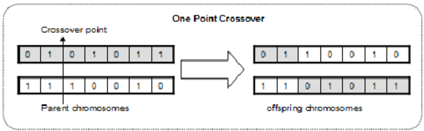
A suitable recombination operator is the so-called one-point
crossover,
where we align two parents,
pick a random point along their length.
Then at that point, exchange the tails,
creating two new offspring.
This is not necessarily optimal, but it works.
Probability
We will apply this with 70% probability, i.e.,
for each pair of parents,
there is a 70% chance that we will create two offspring by
crossover,
and 30% that the children will be just copies of the parents.
A suitable mutation operator is so-called bit-flipping:
in each position we invert the value with a small probability,
pm sampled in the range [0, 1).
Probability
Mutation rate of pm = 1/n
On average that will change about one bit value in every
offspring.
A bit is seen as an allele value for a single gene.
For example, 1/500 chance for any given base, for a population of
500.
import random

for i in range(len(individual_genome), n):
    chance = random.random()  ## (0, 1]
    if chance < 1 / n:
        # xor with 1 to flip bit:
individual_genome[i] = individual_genome[i]^1In this case we will create the same number of offspring as we have
members in our initial population.
Population size: 500
Number of offspring: 500
Parent and survival:
We will use a tournament for selecting the parents:
We pick two members of the population at random (with
replacement).
The one with the highest value q(p) wins the tournament and becomes a
parent.
Generational scheme for survivor selection:
All of the older population in each iteration are discarded,
and parents replaced by their offspring.
For our initial population,
for each position of the genome,
random choice of 0 and 1.
In this case, we do not know the maximum value that we can
achieve.
We will run our algorithm until no improvement in the fitness,
of the best member of the population,
has been observed for 25 generations.
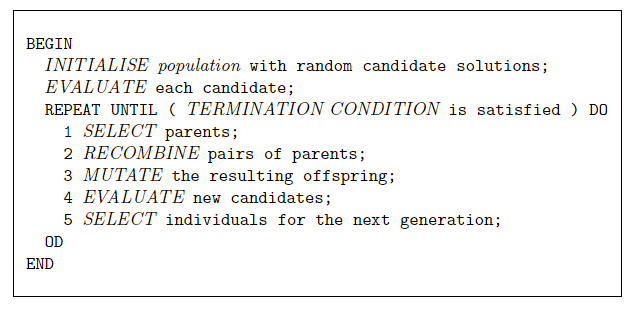
Our evolutionary algorithm to tackle this problem can be specified as below:
Remember:
The following major parts are to be defined for each problem to be
solved:
Discussion questions:
Which of the above parts do you think is the computational bottleneck,
why?
Which of the above parts is the design (human creativity/difficulty)
bottleneck, why?
+++++++++++++++ Cahoot-03-1
Progression in optimizing on a 1-dimensional fitness landscape:
Early stage:
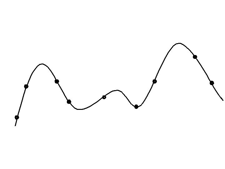
Quasi-random initial population distribution
Mid-stage exploration:
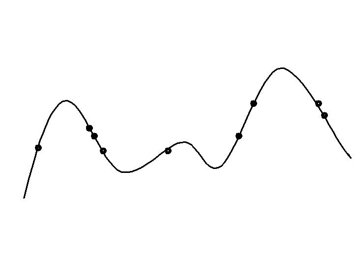
Population starts to arrange around/on hills.
Late stage exploitation:
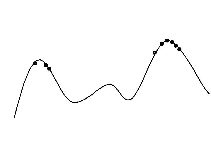
Population concentrated on high hills.
What is the “Memory” of GA?
Each string has a goodness (fitness) or optimality.
This value determines its future influence on search process,
i.e., survival of the fittest.
Solutions which are good, are used to generate other,
similar solutions which may also be good (or even better).
The population at any time stores all we have learned about the
solution,
accessible at any point.
You just access a good individual.
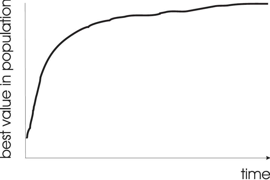
Typical run of an EA shows so-called “anytime behavior”.
Answer:
It depends on how much you want the last bit of progress.
It may be pragmatically better to do more short runs,
with more time spend achieving rapid, effecient returns.
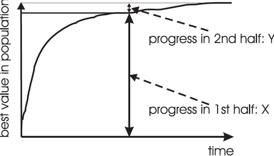
This is the notion of:
https://en.wikipedia.org/wiki/Diminishing_returns
Continued cost for less and less benefit likely has diminishing
practical utility,
though it may yield marginally better solutions.
Discuss:
Are all problems going to show progressive improvement?
Might some runs demonstrate insight,
or sudden bursts of discovery?
Would this same principle apply in such situations?
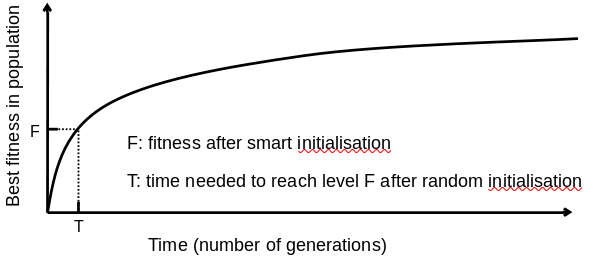
Answer: it depends.
Possibly good, if good solutions/methods exist.
Care is needed, see upcoming lectures on hybridization.
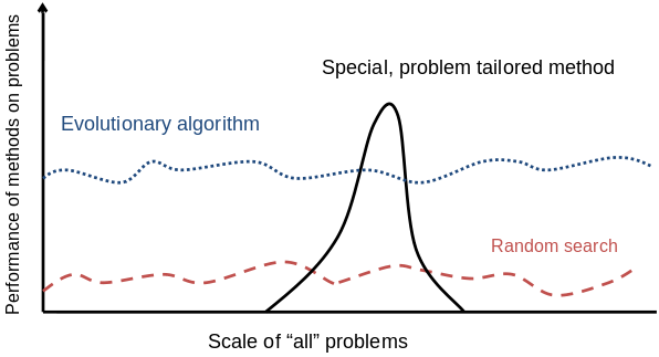
There are many views on the use of EAs as robust problem solving
tools.
For most problems a problem-specific tool may:
perform better than a generic search algorithm on most instances,
but not do well on all instances.
Goal is to provide robust tools that provide:
evenly good performance,
and do so over a wide range of problems and instances.
Goldberg view (1989)
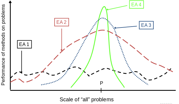
Trend in the 1990’s:
Add problem specific knowledge to EAs,
(special variation operators, repair, etc).
Result: EA performance curve “deformation”:
better on problems of the given type,
worse on problems different from given type,
amount of added knowledge is variable.
Some recent learning and information theory suggests trade-offs,
where the search for an “all-purpose” algorithm may be of limited
utility.
Discussion questions:
Do you think we discover a learning rule so general,
that it can match human generality?
Do you think it might have constraints,
in how it must be taught/handled/babied/trained to perform well?
Any intuition for what they may be?
Michalewicz view (1996)
Global optimization problems:
search with goal of finding the best solution, _x*,_
out of some fixed set of solutions, S.
Deterministic approaches (classic AI):
Guarantee to find an optimal solution, _x*._
Complete enumeration of all s in S,
is guaranteed to be globally optimal…
but it’s brute force.
Can also order search through S.
e.g. box decomposition (branch and bound, etc)
May have bounds on run-time, usually super-polynomial
Heuristic Approaches (extensions to classic
AI):
Cull the search space (and then generate and test).
Some estimation heuristic, helps to search the random space in a more
directed way.
Must decide on some heuristic rules for deciding which x in S to
generate next.
No bounds on run-time.
For some randomized heuristics, such as simulated annealing,
convergence proofs do in fact exist,
i.e., they are guaranteed to find _x*_ in many cases.
Unfortunately these algorithms are fairly weak,
in the sense that they will not identify _x*_ as being globally
optimal,
rather as simply the best solution seen so far.
Let’s think about:
“I don’t care if it works as long as it converges”
vs.
“I don’t care if it converges as long as it works”
We can also use operators that impose some kind of structure onto the
elements of S,
such that each point x has associated with it a set of neighbors N
(x).
In our “landscape” the variables (traits) x and z were taken to be
real-valued,
which imposes a natural structure on S.
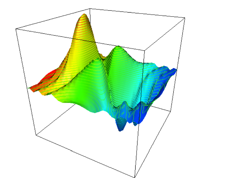
This looks like a continuous outcome above.
However, genomes may not always produce continuous fitness
interpretations of the genome.
For example combinatorial optimization (int or binary genomes) can
produce discontinuous spaces.
Imagine optimizing something more like this:
https://en.wikipedia.org/wiki/Ackley_function
Many heuristics impose a neighborhood structure on search space,
S.
Such heuristics may guarantee that best point found is locally
optimal,
e.g. Hill-Climbers.
Often heuristics very quick to identify good solutions.
But, problems often manifest as local optima.
Question:
What is the neighborhood in an EA?
What part of the meta-heuristic moves the search through the
neighborhood with EC?
Is the entire search space reachable by any heuristic algorithm?
EAs are distinguished by:
Probability distributions over the neighborhood structure:
The breeding population provides the algorithm with change,
a means of defining a nonuniform probability distribution function
(p.d.f.),
governing the generation of new points from an existing S.
This p.d.f. reflects possible interactions between points in S,
which are currently represented in the population.
The interactions arise from the recombination of partial
solutions,
from two or more members of the population (parents).
This potentially complex p.d.f. contrasts with:
the lack of any probability distribution in deterministic solvers,
the globally uniform distribution of blind random search, and
the locally uniform distribution used by many heuristic or stochastic
algorithms,
such as simulated annealing, and various hill-climbing algorithms.
The ability of EAs to maintain a diverse set of points,
provides not only a means of escaping from local optima,
but also a means of coping with large and discontinuous search
spaces.
In addition, as will be seen later,
if several copies of a solution can be generated, evaluated, and
maintained in the population,
this provides a natural and robust way of dealing with problems,
where there is noise or uncertainty,
associated with the assignment of a fitness score to a candidate
solution.
Implicit parallelism:
Each evaluation provides information on many possible candidate
solutions.
Modularity:
Class example, does crossing over help more with modular templates or
with non-modular templates?
To generate something like the phrase in your first assignment:
“methinks it is like a weasel”
from a random sample of a paragraph in English,
or from that same sample with letters randomized.
Which is faster?
Building blocks:
“Short, low-order, and highly fit schemata are sampled, recombined, and
re-sampled,
to form strings of potentially higher fitness…
we construct better and better strings,
from the best partial solutions of the past samplings.”
– David Goldberg, 1989
T. Bäck. Evolutionary Algorithms in Theory and Practice. Oxford
University Press, New York, 1996
U. Bäck, H.-P. Schwefel. An overview of Evolutionary Algorithms for
parameter optimisation. Evolutionary Computation, 1:1 pp. 1–23, 1993.
One of the first papers to really unify historically isolated strands of
EA research within a common framework.
A.E. Eiben. Evolutionary computing: the most powerful problem solver in
the universe? Dutch Mathematical Archive (Nederlands Archief voor
Wiskunde), 5/3:2 pp. 126–131, 2002
Available at http://www.cs.vu.nl/~gusz/papers/ec-intro-naw.pdf
D.B. Fogel. Evolutionary Computation. IEEE Press, 1995
M.S. Hillier, F.S. Hillier. Conventional optimization techniques.
Chapter 1, pp. 3–25 in Sarker et al., Eds. Evolutionary Optimization,
Kluwer Academic Publishers, Boston. 2002. Provides a background on other
methods to place EC in context
X.~Yao. Evolutionary computation: A gentle introduction. Chapter 2,
pp.~27–53 in Sarker et al., Eds. Evolutionary Optimization, Kluwer
Academic Publishers, Boston. 2002.