1 04-RepresentMutateRecombine

Previous: 03-MetaheuristicParts.html

• Cahoots
• Discussion questions
• More images
• More detailed/concrete examples, code
• Simplify and reduce text more

1.1 Representation

“The formulation of the problem is often more essential than its solution.”
-Albert Einstein

In EC, the representation is hard,
but that’s actually a good thing!

1.2 Representation, Mutation, and Recombination

1.2.1 Goals

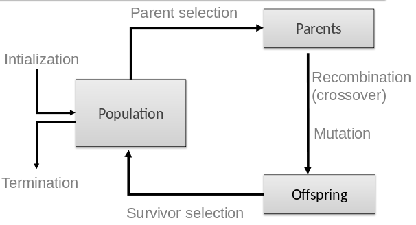
Cover the role of representation and variation operators.

Review the most common representation of genomes:

• Binary
• Integer
• Real-Valued or Floating-Point
• Permutation
• Tree
• FSM (discussed more later, not in this lecture)

You don’t have to stick to the common representation schemes.
One can used hybrid, custom, and mixed representations and operators,
depending on the problem.

1.2.2 Reminder: General scheme of EAs

1.2.3 Role of representation and variation operators

The first stage of building an EA and most cognitively difficult one:

Choose the correct representation for the problem.
It’s not the most computationally difficult (that’s often fitness for large pop).

With a given representation,
one must also choose variation operators:
Mutation and Crossover
The type of variation operators needed depends on chosen representation!

1.2.4 Mutation (1 parent)

https://en.wikipedia.org/wiki/Mutation_(genetic_algorithm)
Mutation uses only one parent and creates one child.
Applies some kind of randomized change to the representation (genotype).
The form taken depends on the choice of encoding used.
One usually also chooses an associated parameter,
which is introduced to regulate the intensity or magnitude of mutation.
Depending on the given implementation, this can be:
mutation step size, etc.
mutation probability,
mutation rate,

1.2.4.1 Rate

No matter the representation, there is usually a measure of mutation rate, p_m.
Usually mutation rate (or quantity) is low.

For this lecture, we concentrate on the choice of operators,
rather than of parameters.
Parameters can make a significant difference in the behavior of the evolutionary algorithm.
This is discussed in more depth later in the class:
07-ParameterTuning.html
08-ParameterControl.html

1.2.5 Recombination (2+ parent)

https://en.wikipedia.org/wiki/Crossover_(genetic_algorithm)
From the information contained within two (or more) parent solutions,
a new individual solution is created.

1.2.5.1 Distinguishing feature of EC: Recombination

Different branches of EC historically emphasized different variation operators.
As these came together under the umbrella of evolutionary algorithms,
this emphasis prompted a great deal of debate.
A lot of research activity has focused on recombination,
as the primary mechanism for creating diversity.
Mutation is sometimes considered as a background search operator.
Combining partial solutions via recombination distinguishes EAs from other global optimization algorithms.

1.2.5.2 Crossover?

The term recombination has come to be used for the more general case.
Early authors used the term crossover,
motivated by the biological analogy to meiosis.
Therefore we will occasionally use the terms interchangeably.
Crossover tends to refer to the most common two-parent case.

1.2.5.2.1 Rate

Recombination operators are usually applied probabilistically,
according to a crossover rate p_c which defines whether recombination happens.

Usually two parents are selected,
and with with probability p_c
two offspring are created via recombination of the two parents.
Or, with probability 1 - p_c
simply copy the parents,

Usually recombination rate (or quantity) is high.

Discuss:
Why can recombination rate be high, but mutation rate not?

1.3 Binary Representation

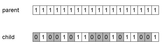
One of the earliest representations.
Genotype consists of a string of binary digits.

In choosing the genotype-phenotype mapping for a specific problem,
one should ideally make sure that the encoding allows both:

1. that all possible bit strings denote a valid solution to the given problem, and
2. that, vice-versa, all possible solutions can be represented.

For some problems, particularly those concerning Boolean decision variables,
the genotype-phenotype mapping is natural.

Using 0-1 bit-strings to encode non-binary information is usually a mistake,
and better results can be obtained by using the integer, real-valued, or other representations directly!

As an extreme example, one could mutate a binary code file using 0s and 1s,
but the probability that you generate valid code is near 0!
It’s better to use Lisp strings!

Why?
Constraints are best specified at the level of abstraction you are searching at!
Like with n-queens, or knapsack, we want to reduce the search space in choosing our encoding.
Choosing a representation at too high a level of abstraction can make the solution unreachable.
Choosing a representation at too low a level of abstraction can unnecessarily increase our search space.

1.3.1 Mutation

The most common mutation operator for binary encodings considers each gene (position/bit) separately,
and allows each bit to flip (i.e., from 1 to 0 or 0 to 1).
Probability of mutation at each gene is p_m,
also called the mutation rate.
Most binary coded GAs use mutation rates in a parameterized range,
such that on average between one gene per generation and one gene per offspring is mutated.
Typically mutation rate is between 1/pop_size and 1/chromosome_length.

Cautionary note:
If you choose a binary representation when you should have chosen a higher level representation,
mutation can cause variable effect!
e.g., If the goal is to evolve an integer number,
you would like to have equal probabilities of changing a 7 into an 8 or a 6.
However, changing 0111 to 1000 requires four bit-flips while changing it to 0110 takes just one.
Thus, the probability of changing 7 to 8 is much less than changing 7 to 6.
Use gray coding to fix such issues,
or just use a different interpretation or representation entirely…

Q: Which do you want more:
one good individual, or
a good population?

A: If one good individual is desired, then choose slightly higher mutation rate
A: If a population is desired, then choose slightly lower mutation rate

What if you’re:
losing diversity?
not converging?
These are all parameter tuning issues for later!

1.3.2 Crossover

1.3.2.1 1-point crossover

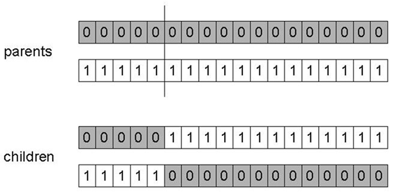
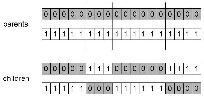
Choose a random point on the two parents,
with length l, and random position r:
r = random(1, l -1)
This limit keeps it away from the far ends.
Split parents at this crossover point.
Create children by exchanging tails.
Typically in range of probability:
p_c = [0.6, 0.9]

1.3.2.2 Alternative Crossover Operators

Why do we need other crossover(s)?
Performance with 1-point crossover depends on the order that variables occur in the representation.
It is more likely to keep together genes that are near each other.

Side note:
In biology, this is also true!
Genes close by each other are likely inherited together.
This is actually how we first started mapping chromosomes!

1-point can never keep together genes from opposite ends of string.
This is also true for odd n-point crossover (below).
This is known as Positional Bias.

Biases like this can be both good and bad!
If we know about the structure of our problem,
they can be exploited for modular use.
But, we do not always understand the structure of information in our problem domain.

Side note:
Understanding the structure of information in your problem domain is important generally!

What if we allow evolving our encoding itself?
For example, to allow genes to switch positions?
Might functional gene assemblies move toward each other more over evolutionary time?
Might functional gene assemblies move apart from each other less over evolutionary time?

1.3.2.3 n-point crossover

Choose n random, independent crossover points:
r₁ = random(1, l-1)
r₂ = random(1, l-1)
…
r_n = random(1, l-1)
Split along those points.
Glue parts, alternating between parents.
Generalization of 1-point.

Still has some positional bias, but less.
This has both pros and cons,
depending on the mapping of the representation domain,
to the material problem domain.

1.3.2.4 Uniform crossover

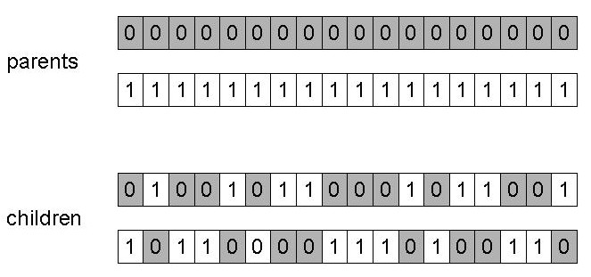
Treat each gene independently,
and make a random choice as to which parent it should be inherited from.
Uniform distribution over [0,1].
Assign ‘heads’ to one parent, ‘tails’ to the other.
Flip a coin for each gene of the first child.
Make an inverse copy of the gene for the second child.
Inheritance is independent of position.

When n-point is odd (e.g., one-point crossover),
there is a strong bias against keeping together certain combinations of genes,
that are located at opposite ends of the representation.
These effects are known as positional bias.

This is extensively studied from both a theoretical and experimental perspective.
This uniform method breaks ties between positions.
Uniform crossover does have a strong tendency towards transmitting 50% of the genes from each parent,
and against transmitting an offspring with a large number of co-adapted genes from one parent.
This is known as distributional bias.

We no longer capitalize on modularity to the same degree.
Which may or may not matter, depending on the encoding.

Discuss:
This is still better than pure mutation.
Why?

1.3.3 Positional versus distributional bias?

It is not usually easy state that one or the other of these operators performs best on any given problem.
An understanding of the types of bias exhibited by different recombination operators can be valuable,
when designing an algorithm for a particular problem,
particularly if there are known patterns or dependencies in the chosen representation,
that can be exploited.

1.3.3.1 Postional

To use the knapsack problem as an example,
it might make sense to use an operator that is likely to keep together the decisions for the first few heaviest items.
If the items are ordered by weight (cost) in our representation,
then we could make this more likely by using n-point crossover,
with its positional bias.

1.3.3.2 Distributional

However, if we used a random weight ordering during knapsack encoding,
then this might actually make it less likely that co-adapted values for certain decisions were transmitted together,
so we might prefer uniform crossover.

1.3.4 Crossover OR mutation?

Decade long debate:
which one is better / necessary / redundant?

Answer (at least, rather wide agreement):
it depends on the problem, but
in general, it is good to have both
Each have a different role.
Mutation-only-EA is possible.
Crossover-only-EA does not work with binary strings.
Why?
But, Crossover-only-EA may work with other representations.

1.3.4.1 Exploration versus Exploitation

A very general principle of learning agents under pressure.
There is co-operation AND competition between each.

1.3.4.1.1 Exploration:

Discovering promising areas in the search space,
i.e. gaining information on the problem.
To some extent, crossover is more exploratory,
as it makes a big jump to an area somewhere “in between” two (parent) areas.
For binary strings, only mutation can introduce new information (alleles).
For other representations, recombination can introduce new information too.

1.3.4.1.2 Exploitation:

Optimizing within a promising area, i.e. using information.
To some extent, mutation is more exploitative,
as it creates random small diversions,
thereby staying near (in the area of) the parent.

Only crossover can combine information from two parents.
For binary strings, crossover does not change the allele frequencies of the population.
Thought experiment:
50% 0’s on first bit in the population,
?% after performing n crossovers.

Early on in the search process,
recombination makes rapid progress.
To hit the final optimum you often need a ‘lucky’ mutation.

1.4 Integer Representation

Now it is generally accepted that it is better to encode directly,
with numerical or discrete variables in the problem domain,
directly as numerical representations (integers, floating point variables).
Many problems naturally have integer variables,
e.g. image processing parameters.

For integer problems,
we want to find the optimal values for a set of variables that all take integer values.
These values might be either:

unrestricted
(i.e., any integer value is permissible),

Restricted to a finite set:
for example, if we are trying to evolve a path on a square grid,
we might restrict the values to the set {0,1,2,3}
representing {North, East, South, West}.

You could also consider this a string representation.
Would it matter?
How are strings encoded?
The representation is 1:1 (the same level of abstraction).
Strings can be considered a case of integer representation.

To decide whether to use an integer representation, we ask:
are there any natural relations between the possible values that an attribute can take?
This might be obvious for ordinal attributes such as integers
(2 is more like 3 than it is 389),
But, for cardinal attributes such as the compass points above,
there may not be a natural ordering.
In either case an integer encoding is probably more suitable than a binary encoding!

One example includes categorical values from a fixed set,
e.g. {blue, green, yellow, pink}
To give a well-known example of where there is no natural ordering,
let us consider the graph k-coloring problem.
Here we are given a set of points (vertices),
and a list of connections between them (edges).
The task is to assign one of k colors to each vertex,
so that no two vertices, which are connected by an edge, share the same color.
For this problem there is no natural ordering:
‘red’ is no more like ‘yellow’ than ‘blue’,
as long as they are different.
We could assign the colors, to the k integers representing them, in any order,
and still get valid equivalent solutions.

1.4.1 Mutation

For integer encodings, there are two principal forms of mutation used:

Random resetting
Creep mutation

Both mutate each gene independently,
with user-defined probability, p_m

1.4.1.0.1 Random resetting

Here the logic of the bit-flipping mutation of binary encodings,
is extended to create random resetting.
Preferable for many categorical variables
(of which strings are a case).
For example, random resetting is the most suitable operator to use,
when the genes encode for cardinal attributes like direction,
or categorical values from a set like color.
This is because all other gene values are equally likely to be chosen.

Rate, probability
In each position independently, with probability p_m,
a new value is chosen at random from the set of permissible values.
The probability distribution over fixed elements can be uniform, or not, and is flexible.

1.4.1.0.2 Creep mutation

This scheme was designed for ordinal attributes (where value, order is meaningful).
Works by adding a small (positive or negative) value to each gene with probability p.
Usually these values are sampled randomly for each position,
from a distribution that is symmetric about zero,
and is more likely to generate small changes than large ones.

Rate, probability
It should be noted that creep mutation requires a number of parameters,
controlling the distribution from which the random numbers are drawn,
and hence the size of the steps that mutation takes in the search space.
Finding appropriate settings for these parameters may not be easy,
and it is sometimes common to use more than one mutation operator in tandem from integer-based problems.
For example, both a “big creep” and a “little creep” operator are sometimes used.

Alternatively, random resetting might be used with low probability,
in conjunction with a creep operator that tended to make small changes,
relative to the range of permissible values.

1.4.2 Recombination

Just re-use the binary recombination operations:
When each gene has a finite number of possible allele values, such as integers,
it is normal to use the same set of operators as for binary representations.
That’s easy!

These operators are valid:
The offspring can not fall outside the given genotype space.

These operators are also sufficient:
We usually want the discrete variables,
and it usually does not make sense to consider ‘blending’ allele values.
For example, even if genes represent integer values,
averaging an even and an odd integer yields a non-integral result.

1-point

n-point

Uniform

1.5 Real-Valued or Floating-Point Representation

Often the values that we want to represent as genes,
come from a continuous rather than a discrete distribution.
Many problems naturally occur as real valued problems.
For example, continuous parameter optimization,
where a gene might represent physical quantities such as:
the length, width, height, or weight,
of some component of a design,
that can be specified within a tolerance smaller than integer values.

Satellite boom:
A good example would be the satellite dish holder boom described earlier,
where the design is encoded as a series of angles and spar lengths.

Evolve weights in an ANN:
Another example might be if we wished to use an EA to evolve the weights on the connections between the nodes in an artificial neural network:
https://en.wikipedia.org/wiki/Neuroevolution

A vector (or string) of real values:
A string of real values can sensibly represent a solution to these problems.
The genotype for a solution with k genes is now a vector:
\(<x_1,...,x_k> x_i \ with \in \mathbb{R}\)

The precision of these real values is limited by the implementation,
so clearly we operate using floating-point numbers in code.

Illustration: Ackley’s function (often used in EC)

1.5.1 Mapping real values on bit strings

https://en.wikipedia.org/wiki/Floating-point_arithmetic

How are floats encoded architecturally?

I’ll gloss over this in class:
\(Z \in [x,y] \subseteq \mathbb{R}\) is represented by \(\{a_1, ..., a_L\} \in \{0,1\}^L\)
\([x,y] \rightarrow \{0,1\}^L\) must be invertible (one phenotype per genotype)
\(\Gamma: [x,y]^L \rightarrow [x,y]\) defines the representation:
\(\Gamma (a_1, ...,a_L) = x + \frac{y-x}{2^L -1} (\sum_{j=0}^{L-1}a_{L-j}) \in [x,y]\)
Only 2^L values out of infinite are represented.
L determines possible maximum precision of solution.

But, note that:
High precision usually means slower computations.

1.5.2 Mutation

We consider the allele values as coming from a continuous,
rather than a discrete, distribution.
Thus, the forms of mutation described above are no longer applicable.

It is common to change the allele value of each gene randomly within its domain given by a lower L_i and upper U_i bound:
\(<x_1, ..., x_n> \rightarrow <x'_1, ..., x'_n>, where\ x_i,x'_i \in [L_i, U_i]\)

We assume here that the domain of each variable is a single interval:
\([L_i, U_i] \subseteq \mathbb{R}\)

Like integer representations,
two types can be distinguished by probability distribution,
from which the new gene values are drawn:

1. Uniform
2. Non-uniform mutation.

1.5.2.1 Uniform Mutation

Analogous to bit-flipping (binary) or random resetting (integers).
The values of x’_i are drawn randomly with a uniform distribution from [L_i, U_i].
Like binary and integer, these are normally used with a position-wise mutation probability, p_m

1.5.2.2 Non-uniform mutations

Most schemes are probabilistic.
Usually only make a small change to each gene value.

Small adjustments
One common form is analogous to the creep mutation for integers.
Usually, but not always, the amount of change introduced is small.

Add to the current gene value,
an amount drawn randomly from a Gaussian distribution,
with mean zero and user-specified standard deviation.

\(N(0,\sigma)\) specifies a sample from a normal distribution,
and paramaterizable standard deviation.

Updates as follows:
\(x'_i = x_i + N(0,\sigma)\)
then curtail the resulting value to the range [L_i, U_i] if necessary.

Size of adjustment
Standard deviation, \(\sigma\)
a.k.a, mutation step size, controls amount of change
2/3 of draws will lie in range \((-\sigma \ to\ +\sigma)\)

With Gaussian, probability of drawing a random number,
with any given magnitude, is a rapidly decreasing from zero,
as a function of the standard deviation parameter, \(\sigma\)

Approximately two thirds of the samples drawn,
will lie within plus or minus one standard deviation.
So, most of the changes made will be small.
The tail of the distribution never reaches zero
So, there is nonzero probability of generating very large changes,

\(\sigma\) determines the extent to which given values,
x_i are perturbed by the mutation operator.
Thus, it is often called the mutation step size.
It is common to apply this operator with probability, 1 per gene, p_m=1.
Instead of infrequent application,
the mutation parameter is used to control the standard deviation of the Gaussian,
and hence the probability distribution of the step sizes taken!

The Gaussian:
https://en.wikipedia.org/wiki/Normal_distribution
\(p(\Delta x_i)={\frac {1}{\sigma {\sqrt {2\pi }}}}e^{-{\frac {1}{2}}\left({\frac {\Delta x_i-\epsilon }{\sigma }}\right)^{2}} with\ \epsilon=0\)
Side note:
In general form, \(\epsilon\) would normally be \(\mu\), the mean.
Here, it’s 0.

1.5.2.2.1 Self-Adaptive Mutation

Different mutation strategies (rates),
may be appropriate in different stages of the evolutionary search process,
or different parts of the landscape.

How to adapt step-sizes?

All representations:
As a side note, this self-adaptation sub-section is not just for real/float,
or non-uniform floats, but for many types of representation.
This has been successfully demonstrated in many domains,
not only for real-valued representation,
but also for binary and integer search spaces.

Put step size in genome:
Mutation step sizes are not always set by the user.
\(\sigma\) can also be included in the genome \(<x_1, ..., x_n, \sigma>\)

Thus, step size can undergo variation and selection.
And, it can co-evolve with the solutions,
with all genes/alleles specified together as the vector, \(\bar{x}\)

Net mutation effect: \(<\bar{x}, \sigma> \rightarrow <\bar{x}', \sigma'>\)

Order of evaluation:

First modify the value of \(\sigma\)
\(\sigma \rightarrow \sigma'\)

Then, mutate each x_i value with the new value \(\sigma'\)
\(x \rightarrow x' = x + N(0, \sigma')\)

Thus, a new individual \(<\bar{x}',\sigma'>\) is effectively evaluated twice (a good thing).

First, it is evaluated directly for its viability,
during survivor selection based on \(f(\bar{x}')\)
If \(f(\bar{x}')\) is good, implies \(\bar{x}'\) is good

Second, it is evaluated for its ability to create good offspring.
If the \(\bar{x}'\) is good,
then this implies the new \(\sigma'\) that created it is good

If the offspring generated by using \(\bar{x}'\)
prove viable (in the first sense),
then a given step size that created it, evaluates favorably.

An individual \(<\bar{x}',\sigma'>\) represents both a good \(\bar{x}'\) that survived selection,
and a good \(\sigma'\) that proved successful in generating this good \(\bar{x}'\) from \(\bar{x}\).

Assumptions
Assume that under different circumstances,
different step sizes will behave better than others.

Time and step size
Distinguish different stages within the evolutionary search process,
and guess about the value of different mutation strategies,
which would be appropriate in different stages.
As the search is proceeding,
self-adaptation adjusts the mutation strategy.

Space and step size
The shape of the fitness landscape in its neighborhood,
determines what good mutations are.
Those that jump more into the direction of fitness, increase.

Assigning a separate mutation strategy to each individual,
which co-evolves with it,
opens the possibility to learn and use a better mutation operator,
suited for the local topology.
E.g., more caution on a steep hill, or speed on a flat section.

State of the art: self-adaptation works
Self-adaptive mutation mechanisms have been used,
and have been studied for decades in EC.
Experimental evidence shows that EA with self-adaptation,
outperforms the same algorithm without self-adaptation.
Theoretical results also show that self-adaptation works.

For simple objective functions,
theoretically optimal mutation step sizes can be calculated
in light of some performance criterion,
e.g., progress rate during a run,
and compared to step sizes obtained during a run of the EA in question.

For complex problems and/or algorithms,
a theoretical analysis is usually infeasible.

Time-decay
For a successful run, the step size, \(\sigma\), often ideally decreases over time.
Theoretical and experimental results agree on this observation.
In the beginning of a search process,
a large part of the search space has to be sampled in an exploratory fashion,
to locate promising regions (with good fitness values).
Therefore, large mutations are appropriate in early phase.
As the search proceeds and optimal values are approached,
only fine tuning of the given individuals is needed
Smaller mutations are required during later search.

Landscape itself changes!
The objective function can change over a run!
This mean the landscape and fitness change.
The evolutionary process aims at a moving target.
Previously well-adapted individuals may now have a low fitness.
Population needs to be re-evaluated, and the search space re-explored.
For the new exploration phase required,
late-stage mutation step sizes may be too low.
Implement an experimental test.
After each change in the objective function,
self-adaptation is able to reset the step sizes.

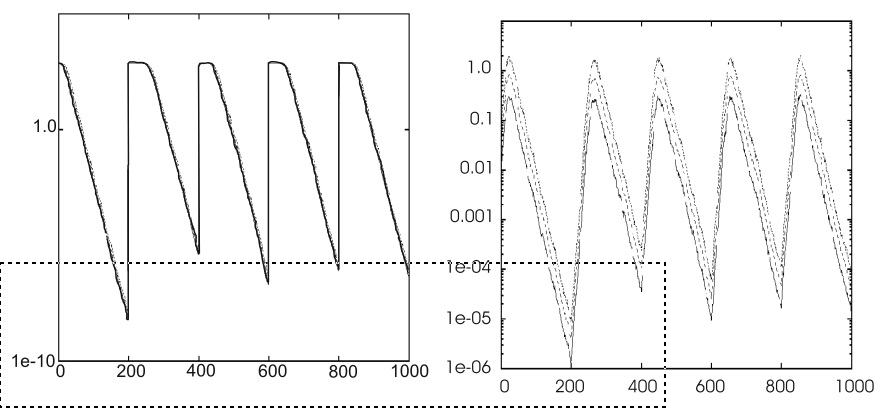
The optimum changes after every 200 generations (generations on x-axes).
Clear effect on the average best objective function values,
(y-axis, left) in the given population.
Self-adaptation adjusts step sizes (y-axis, right).
We see a small delay to increase values,
appropriate for exploring the new fitness landscape, k
As the population approaches the new optimum,
the values of \(\sigma\) start decreasing again.

Conclusions
Much experience has been gained over self-adaptation in Evolutionary Algorithms.
The accumulated knowledge identifies helpful conditions for self-adaptation.

With:
μ - population size
λ - number of offspring

1. μ > 1 so that different strategies are present
2. generation of an offspring surplus: λ > μ
3. a not too strong selective pressure (heuristic: λ / μ = 7, e.g., (15, 100))
4. (μ, λ)-selection (to guarantee extinction of maladapted individuals)
5. recombination, usually intermediate, of strategy parameters

Back to mutation for to float representations:

1.5.2.2.2 Uncorrelated mutation with one step size, σ

Chromosome
\(<x_1, ..., x_n, \sigma>\)

The same distribution, \(\sigma\), is used to mutate each x_i
One strategy parameter \(\sigma\) in each individual.
\(\sigma\) is mutated, each time step.

Multiply it by a term \(e^\Gamma\),
where \(\Gamma\) is a random variable drawn each time,
from a normal distribution with mean 0 and standard deviation \(\tau\).

N(0, 1) denotes a draw from the standard normal distribution
(with stardard deviation 1 instead of parameterizable \(\sigma\)).

N_i(0, 1) denotes a separate draw from the standard normal distribution,
for each variable i .

The proportionality constant \(\tau\) is an external parameter, to be set by the user.
\(N(0, \tau) = \tau \cdot N(0,1)\)

The mutation mechanism for \(\sigma\)
\(\sigma' = \sigma \cdot e^{\tau \cdot N(0,1)}\)

The mutation mechanism, for each x
\(x'_i = x_i + \sigma' \cdot N_i(0,1)\)

The parameter \(\tau\) can be interpreted as a kind of learning rate,
as in neural networks.
It is usually inversely proportional to the square root of the problem size.
\(\tau \propto 1/\sqrt{n}\)

Why mutate with distribution?
The reasons for mutating \(\sigma\) by multiplying with a variable with a lognormal distribution as follows:
Smaller modifications should occur more often than large ones.
Standard deviations have to be greater than 0.
The median (0.5-quantile) should be 1, since we want to multiply the \(\sigma\).
Mutation should be neutral on average.
This requires equal likelihood of drawing a certain value,
and its reciprocal value, for all values.

Lower limit
Standard deviations very close to zero are unwanted.
They will have on average a negligible effect.
The following boundary rule is used to force step sizes to be no smaller than a threshold:
\(\sigma' < \epsilon_0 \Rightarrow \sigma' = \epsilon_0\)
If less than limit, then set to limit.

Example effect on landscape (image)
We have an objective function, \(\mathbb{R}^2 \rightarrow \mathbb{R}\).
Individuals in this example are of the form \(<x, y, \sigma>\).
The mutation step size is the same in each direction.
There are limited points in the search space where new offspring can be placed.
Such placement is drawn as a circle around the individual to be mutated.
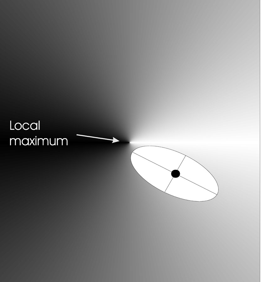
The image below shows the effects of mutation in two dimensions.

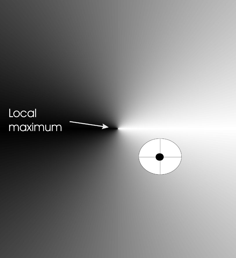
Part of a fitness landscape with a conical shape is shown.
The black dot indicates an individual.
Circle is mutants having the same chance to be created.
Mutation with n = 2, \(n_\sigma\) = 1, \(n_\alpha\) = 0 (angle, more on alpha later).
There is just one \(\sigma\).
Thus, the probability of moving along the y-axis (little effect on fitness),
is the same as that of moving along the x-axis (large effect on fitness)

1.5.2.2.3 Uncorrelated mutation with n step sizes, σ₁-σ_n

Use n step sizes to treat each dimension (gene) differently.

Use different step sizes for different dimensions:
\(i \in \{1, ..., n\}\)

The fitness landscape can have a different slope in one direction (along axis i),
than in another direction (along axis j).

Each basic chromosome:
\(<x_1, ..., x_n>\)

Extend with n step sizes, one for each dimension, resulting in:
\(<x_1, ..., x_n, \sigma_1, ..., \sigma_n>\)

The step size mutation mechanism:
\(\sigma'_i = \sigma_i \cdot e^{\tau' \cdot N(0,1) + \tau \cdot N_i(0,1)}\)

The x mutation mechanism:
\(x'_i = x_i + \sigma'_i \cdot N_i(0,1)\)
where:
\(\tau' \propto 1/2n\)
\(\tau' \propto 1 \sqrt{2\sqrt{n}}\)

A boundary rule is applied to prevent standard deviations very close to zero:
\(\sigma' < \epsilon_0 \Rightarrow \sigma' = \epsilon_0\)

Instead of the individual level (each individual \(\bar{x}\) having its own \(\sigma\)),
it works on the coordinate level (one \(\sigma_i\) for each x_i in \(\bar{x}\)).

The corresponding straightforward modification could be:
\(\sigma'_i = \sigma_i \cdot e^{\tau \cdot N_i(0,1)}\)
Though we use the more complicated one above, for multiple \(\tau\).

The common base mutation \(e^{\tau' \cdot N(0,1)}\) allows for an overall change of the mutability,
guaranteeing the preservation of all degrees of freedom.

The coordinate-specific \(e^{\tau' \cdot N_i(0,1)}\) provides flexibility,
to use different mutation strategies in different directions.

Effect on landscape
The image below shows the effects of mutation in two dimensions.
We have an objective function \(\mathbb{R}^2 \rightarrow \mathbb{R}\).
The black dot indicates an individual.
Individuals are of the form \(<x,y,\sigma_x, \sigma_y>\).
Mutation step sizes can differ in each direction (x and y).
The points in the search space where the offspring can be placed,
with a given probability,
form an ellipse around the individual to be mutated.
The axes of such an ellipse are parallel to the coordinate axes,
with the length along axis i proportional to the value of \(\sigma_i\)

1.5.2.2.4 Correlated mutations

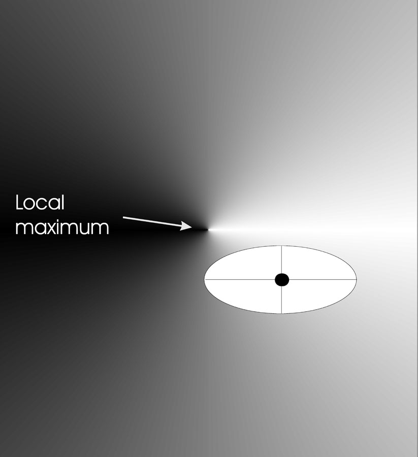
The second version of mutation discussed above,
introduced different standard deviations for each axis,
but this only allows ellipses orthogonal to the axes.
The rationale behind correlated mutations,
is to allow the ellipses to have any orientation,
by rotating them with a rotation (covariance) matrix C.

Comparing our previous two strategies to correlated mutations:

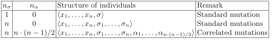
Possible settings of \(n_{\sigma}\) (step) and \(n_{\alpha}\) (angle),
for previous two mutation operators (row 1, 2),
and correlated on row 3.

The image below shows the effects of correlated mutations in two dimensions:

Correlated mutation: n = 2, \(n_{\sigma}\) = 2 (step), \(n_{\alpha}\) = 1 (angle).
The black dot indicates an individual.
The individuals now have the form
\(<x, y, \sigma_x, \sigma_y, \alpha_{x,y}>\)
The points in the search space where the offspring can be placed,
with a given probability,
form a rotated ellipse around the individual to be mutated,
where again the axis lengths are proportional to the \(\sigma\) values.
Points where the offspring can be placed,
with a given probability,
form a rotated ellipse.
The probability of generating a move in the direction of the steepest ascent
(largest effect on fitness) is now larger than that for other directions.

1.5.3 Recombination operators

Three major categories for floats:
1. Discrete
2. Intermediate / Arithmetic
3. Blend

1.5.3.1 Discrete value recombination

Analogous operator to those used for bit-strings,
but now split between floats.
Recombination only gives us new combinations of existing values.

If discrete recombination is used,
then only mutation can insert new values into the population.
This is true of all of the recombination operators described previously.
Each allele value in offspring z,
comes from one of its parents (x, y),
with equal probability:
z_i = x_i or y_i

1.5.3.2 Intermediate/Arithmetic value recombination

Create a new allele value in the offspring,
that lies between those of the parents.
\(z_i = \alpha x_i + (1 - \alpha) y_i \ where \ \alpha: 0 \leq \alpha \leq 1\)

The parameter \(\alpha\) can be either:
constant, uniform arithmetical crossover,
variable, (e.g. depend on the age of the population),
random, every time.
\(\alpha\) serves as a weight between the two parents,
that auto-adjusts to 1.

This form of recombination creates new gene material.
However, as a result of the averaging process,
the range of the allele values in the population for each gene is reduced.

1.5.3.2.1 Single arithmetic recombination

Parents:
\(<x_1, ..., x_n> and \ <y_1, ..., y_n>\)
Pick a single gene (k) at random.
At that position, k,
take the arithmetic average of the two parents.

The other points are copied from the parents.

Child 1:
\(<x_1, ..., x_{k - 1}, \alpha \cdot y_k + (1 - \alpha) \cdot x_k, x_{k + 1}, ..., x_n>\)

Child 2:
The second child is created in the same way,
with x and y reversed.

e.g., k = 8, α = 1/2

1.5.3.2.2 Simple arithmetic recombination

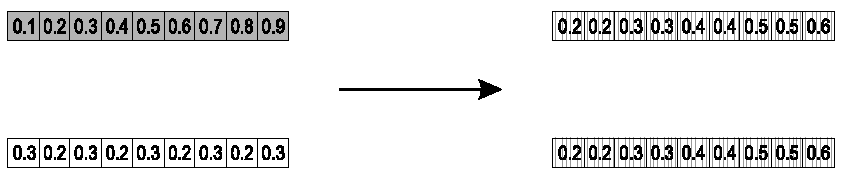
Parents:
\(<x_1, ..., x_n> and \ <y_1, ..., y_n>\)
First pick a recombination point k, after which, mean all values.

Take the first k floats of parents, and put them into the children.
The rest is the arithmetic average of parent 1 and 2.

Child 1:
\(<x_1, ..., x_k, \alpha \cdot y_{k + 1} + (1 - \alpha) \cdot x_{k + 1}, ..., \alpha \cdot y_n + (1 - \alpha) \cdot x_n>\)

Child 2:
The second child is created in the same way,
with x and y reversed.

e.g., with \(\alpha\) = 0.5, k = 6

1.5.3.2.3 Whole arithmetic recombination

This is the most commonly used operator.

Parents:
\(<x_1, ..., x_n> and \ <y_1, ..., y_n>\)
For each gene, take the weighted sum of the two parental alleles.

Child 1 is:
\(\alpha \cdot \bar{x} + (1 - \alpha) \cdot \bar{y}\)

Child 2 is revers:
\(\alpha \cdot \bar{y} + (1 - \alpha) \cdot \bar{x}\)

e.g., with α = 1/2

1.5.3.3 Blend recombination

Create a new allele value in the offspring,
which is close to that of one of the parents,
but may lie outside them.
Child value could be bigger than the larger of the two parent values,
or smaller than the lesser parent.

Can create new material,
without restricting the range.
Create offspring in a region that is bigger,
beyond the n-dimensional rectangle spanned by the parents.

Extra space is often proportional to the distance between the parents.
Parents that are farther apart yields more outer range.

Two parents x and y:
\(<x_1, ..., x_n> and \ <y_1, ..., y_n>\)

For example, in chromosome position i, some value x_i < y_i
The difference is:
d_i = y_i - x_i

To create a child we can sample a random number u uniformly from [0, 1], calculate:
\(\gamma = (1 - 2\alpha)\mu - \alpha\)
and set:
\(z_i = (1 - \gamma) x_i + \gamma y_i\)
Range for the i^th value in the child z is \(z_i = [x_i - \alpha d_i, x_i + \alpha d_i]\)

Interestingly, the original authors reported best results with \(\alpha = 0.5\).
where the chosen values are equally likely to lie inside the two parent values, as outside.
This may balance exploration and exploitation.

1.5.3.4 Comparison between methods

Difference between:
single arithmetic recombination,
whole arithmetic combination, and
Blend Crossover.

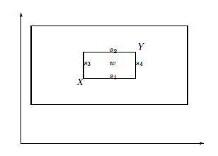
X and Y are individuals (the corners).

Single:
The points {s₁, … , s~4} are four possible offspring,
from single arithmetic recombination with \(\alpha = 0.5\).

Whole:
The single point, w,
is the offspring from whole arithmetic recombination with \(\alpha = 0.5\).

Inner box represents all the possible offspring positions,
as \(\alpha\) is varied.

Blend:
The outer dashed box shows all possible offspring positions,
for blend crossover with \(\alpha = 0.5\),
each position being equally likely.

More recent methods, such as Simulated Binary Crossover,
have built on Blend Crossover,
so that rather than select offspring values uniformly,
from a range around each parent values,
select from a distribution more likely to create small changes,
and the distribution is controlled by the distance between the parents.

1.5.3.5 Multi-parent recombination

We are not constricted by the conservative practicalities of nature!
Mutation uses n = 1 parent.
Traditional crossover n = 2.
Extension to n > 2 is natural to examine.
Been around since 1960s (Prehaps a product of the times, lol…).
Still rare, but studies indicate sometimes useful.

Type 1

• Idea: segment and recombine parents
• Example: diagonal crossover for n parents:
  • Choose n-1 crossover points (same in each parent)
  • Compose n children from the segments of the parents in along a “diagonal”, wrapping around
• This operator generalises 1-point crossover

Type 2

• Idea: arithmetical combination of (real valued) alleles
• Example: arithmetic crossover for n parents:
  • i-th allele in child is the average of the parents’ i-th alleles
• Creates center of mass as child
• Odd in genetic algorithms, long known and used in evolution strategies

1.6 Permutation Representations

Many problems decide on the order of a sequence of events.
Representations define a permutation of a fixed set of values.
Fixed values are typically integers.

1.6.1 Why not binary or integer?

A binary, or simple integer, representation allows numbers to occur more than once.
Such sequences of potentially repeating integers would not represent valid permutations.
Mutation and recombination operators must preserve the unique permutation property.
Each possible allele value must occur exactly once in the solution.

1.6.2 Alternative representations

decoder functions based on unrestricted integer representations,
“floating keys” based on real-valued representations,
etc.

1.6.3 Recall n-queens

Represent each candidate solution as a list of integers.
Each queen was on a different column, or list position.
Each integer value represented the rows on which a queen was positioned.
We required that these be a permutation of unique elements.
Thus, no two queens can share the same row.

1.6.4 Classes

Two classes of permutation problem exist:
order, and
adjacency.

1.6.4.1 Order

Absolute order can determine correctness.
This might happen when the events use limited resources or time.

A typical example is the production scheduling problem.
In which order should a series of products be manufactured on a set of machines?
There may be dependencies between products.
Specifically, there might be different setup times between products.
Further, one product might be a component of another.
For example, it might be better for widget 1 to be produced before widgets 2 and 3,
which in turn might be preferably produced before widget 4,
no matter how far in advance this is done.
In this case it might well be that the sequences [1,2,3,4] and [1,3,2,4] have similar fitness,
and are much better than, for example, [4,3,2,1].

1.6.4.2 Adjacency

Adjacency can define correctness.

A common example is the:
https://en.wikipedia.org/wiki/Travelling_salesman_problem
How do we find a complete tour of n cities, of minimal length?
There are (n-1)! different routes possible, for n given cities.
This includes the asymmetric case, counting back and forth as two routes…
For n = 30 there are approximately 10³² different tours.
We label the cities 1, 2, …, n.
A complete tour is defined by a permutation.
It is the links between cities that are important.
The difference from absolute ordering problems is subtle.
Starting point of a tour is not important.
For example, [1,2,3,4], [2,3,4,1], [3,4,1,2], and [4,1,2,3] are all equivalent.
As we mentioned before, many examples of this class are also symmetric.
To extend the example, [4,3,2,1] is also equivalent.

1.6.5 Encoding

Two possible methods to encode a permutation exist.

We can use an example of four cities:
[A,B,C,D].
A represented permutation, or candidate solution, could be:
[3,1,2,4].

1.6.5.1 Event ID

In the first method,
the i^th element of the representation denotes the event that happens,
in that place in the sequence.

(TSP: the i^th destination visited).
The first encoding denotes one tour of [A,B,C,D] as:
[3,1,2,4] as [C,A,B,D]

1.6.5.2 ID position

In the second method,
the value of the i^th element denotes the position in the sequence,
in which the i^th event happens.

The second encoding denotes one tour of [A,B,C,D] as:
[3,1,2,4] as [B,C,A,D].

Discussion question:
Which method do you find most intuitive?
Do you have any idea why?

1.6.6 Mutation

Mutate one permutation to produce another valid permutation.

Independence
For previous representations, we defined an independent probability that a single gene in the chromosome is altered.
It is longer possible to consider each gene independently.
Now, finding legal mutations requires moving alleles around in the genome.
The mutation parameter is interpreted as the probability that the chromosome undergoes mutation.

Uniqueness
Previously covered mutation operators can lead to inadmissible solutions for permutations.
For example, let gene i have value j.
If we change j to some other value k,
then k would occurr twice,
and j would no longer occur.

We review four methods of mutation for permutation:

Swap,
Insert,
Scramble, and
Inversion.

1.6.6.1 Swap mutation

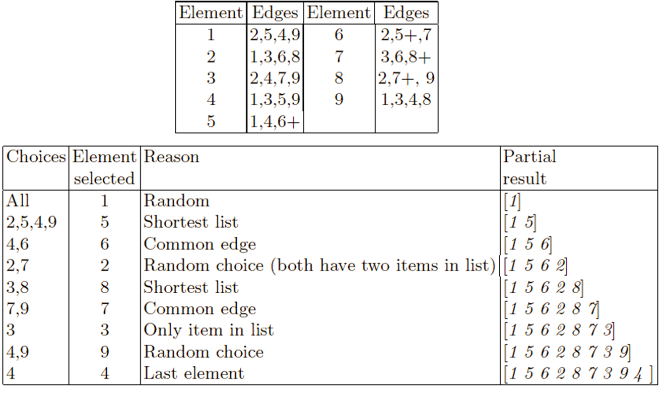
Randomly select two positions (genes) in the chromosome.
Swap allele values.

Image: Positions 2 and 5 were chosen, and swapped.

1.6.6.2 Insert Mutation

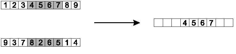
Randomly select two gene positions (allele values).
Shift the second forward, to immediately follow the first.
Shift those between later, to accommodate.
This preserves most of the order, and much adjacency information.

Image: Positions 2 and 5 were chosen, and 5 shifted backward.

1.6.6.3 Scramble mutation

Randomly select a contiguous range of genes.
Randomly re-arrange the alleles in those positions.
If range is large enough, in the limit, this scramble the entire chromosome.

Image: Positions 2-5 were chosen, and randomly permuted.

1.6.6.4 Inversion mutation

The first three operators make small changes,
to the order in which allele values occur.
For adjacency-based problems,
this can cause large numbers of links to be broken.
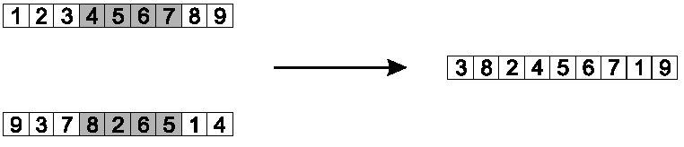
Thus, for adjacency problems, inversion is commonly used.
Inversion reverses a randomly chosen sub-string.

Steps:
Randomly select two positions in the chromosome.
Choosing two positions breaks the chromosome into three parts.
In the middle part, reverse the order in which the values appear.
All links inside each part are preserved.
The two links between the three parts are broken.

This operator is illustrated here:

Image: positions 2-5 were selected, and inverted.

Generalization:
At a range of 2 genes, inversion is the smallest change,
that can be made to an adjacency-based problem.
All other types of changes could be constructed as a series of inversions.
Ordering of the search space induced by this operator,
forms a natural basis for considering this class of problems as a whole.
It is similar to the Hamming space for binary problem representations.
It is also the basic logic behind the 2-opt search heuristic for TSP,
and by extension k-opt:
https://en.wikipedia.org/wiki/2-opt

++++++++++++++ Cahoot 04-n

1.6.7 Recombination operators

Combine 2+ permutation parents,
to produce valid permutation offspring.

1.6.7.1 Problem

For the design of recombination operators,
permutation-based representations present some difficulties.
It is not generally possible simply to exchange sub-strings between parents,
and still maintain the unique permutation property.

What do the solutions actually represent?
an order in which elements occur, or
a set of transitions linking pairs of elements.

1.6.7.2 Solution

Specialized recombination operators must be designed for permutations.
Operators ideally transmit information contained in the parents.
Some emphasize transmitting information in either parent.
Some emphasize transmitting information shared between parents.

Now, we will review the following methods:

Partially mapped crossover (PMX),
Edge recombination,
Order recombination, and
Cycle recombination.

1.6.7.3 Partially Mapped Crossover (PMX)

Procedure for parents P1 and P2:
Choose two crossover points at random.
Copy the segment between them from the first parent (P1) into the first offspring.
Starting from the first crossover point,
look for elements in that segment of the second parent (P2),
that have not been copied.
For each of these (say i),
look in the offspring to see what element (say j),
has been copied in its place from P1.
Place i into the position occupied by j in P2,
since we know that we will not be putting j there
(as we already have it in our string).
If the place occupied by j in P2,
has already been filled in the offspring by an element k,
then put i in the position occupied by k in P2.
Having dealt with the elements from the crossover segment,
the remaining positions in this offspring can be filled from P2.
The second child is created analogously with the parental roles reversed.

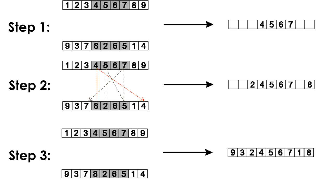
step 1:
copy randomly selected segment from first parent into offspring.

step 2:
consider in turn the placement of the elements that occur in the middle segment of parent 2 but not parent 1.
The position that 8 takes in P2 is occupied by 4 in the offspring,
so we can put the 8 into the position vacated by the 4 in P2.
The position of the 2 in P2 is occupied by the 5 in the offspring,
so we look first to the place occupied by the 5 in P2, which is position 7.
This is already occupied by the value 7,
so we look to where this occurs in P2,
and finally find a slot in the offspring that is vacant, the third.
Finally, note that the values 6 and 5 occur in the middle segments of both parents.

step 3:
copy remaining elements from second parent into same positions in offspring

Preserve what parents share?
Inspection of the offspring created shows that in this case,
six of the nine links present in the offspring,
are present in one or more of the parents.
However, of the two edges {5-6} and {7-8} common to both parents,
only the first is present in the offspring.
Some suggest that a desirable property of any recombination operator is that of parental respect,
i.e., that any information carried in both parents should also be present in the offspring.
This is true for all of the recombination operators described above for binary and integer representations,
and for discrete recombination for floating-point representations,
However, as the example above shows, is not necessarily true of PMX.
Several other operators have been designed for adjacency-based permutation problems:

1.6.7.4 Edge Recombination

Offspring are be created such that its edges are present in at lest one of the parents.
Edge recombination has undergone a number of revisions over the years.
Here we show a design that ensures common edges are preserved.
Using the two parents, an edge table is constructed.
This edge table is also known as an adjacency list.
For each element, it lists the other elements that are linked to it, in the two parents.
Marking a ‘+’ in the table indicates that an edge is present in both parents.
The operator works as follows:

Construct a table listing which edges are present in the two parents.
If an edge is common to both, mark it with a +.

For example, parents:
[1 2 3 4 5 6 7 8 9] and [9 3 7 8 2 6 5 1 4]

Start randomly.
Pick an initial element, entry, at random, and put it in the offspring.
Set a variable, current_element=entry.
Remove all references to current_element from the table.
Examine edge list for current_element.
If there is a common edge (+),
then pick that to be next element.
If not,
then pick the entry in the list which itself has the shortest list.
Split ties at random.
In the case of reaching an empty list,
the other end of the offspring is examined for extension.
Otherwise, a new element is chosen at random.
Only in the last case, will so-called foreign edges be introduced.

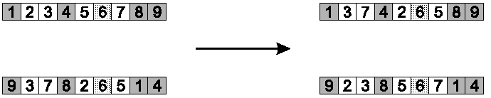
Edge-3 recombination is illustrated by the following example.
The parents are the same two permutations used in the PMX example:
[ 1 2 3 4 5 6 7 8 9] and [ 9 3 7 8 2 6 5 1 4].

Note that only one child per recombination is created by this operator.

1.6.7.5 Order 1 crossover

This operator begins in a similar fashion to PMX.
It copies a randomly chosen segment of the first parent into the offspring.
However, it proceeds differently.
The intention is to transmit information about relative order from the second parent.
Next, choose two crossover points at random.
Copy the segment between them from the first parent (P1) into the first offspring.
Starting from the second crossover point in the second parent,
copy the remaining unused numbers into the first child,
in the order that they appear in the second parent,
wrapping around at the end of the list.
Create the second offspring in an analogous manner, with the parent roles reversed.

Copy randomly selected set from first parent:

Copy the rest from second parent, in order 1,9,3,8,2

Summary

• Idea is to preserve relative order that elements occur.
• Informal procedure:
• 1. Choose an arbitrary part from the first parent
• 2. Copy this part to the first child
• 3. Copy the numbers that are not in the first part, to the first child:
  • starting right from cut point of the copied part,
  • using the order of the second parent
  • and wrapping around at the end
• 4. Analogous for the second child, with parent roles reversed

1.6.7.6 Cycle recombination

Preserves as much information as possible about the absolute position in which elements occur.
A cycle is a subset of elements that has the following property:
Each element always occurs paired with another element of the same cycle when the two parents are aligned.
Notice the three example cycles below.
Then, re-read that definition above.

Divide the elements into cycles.
Select alternate cycles from each parent, to create offspring.
The procedure for constructing cycles is as follows:
1. Start with the first unused position and allele of P1.
2. Look at the allele in the same position in P2.
3. Go to the position with the same allele in P1.
4. Add this allele to the cycle.
5. Repeat steps 2 through 4 until you arrive at the first allele of P1.

Step 1: identify cycles

Three cycles were identified.

Step 2: copy alternate cycles into offspring

Summary

• Each allele comes from one parent together with its position.
• Informal procedure:

1. Make a cycle of alleles from P1 in the following way.
   1. Start with the first allele of P1.
   2. Look at the allele at the same position in P2.
   3. Go to the position with the same allele in P1.
   4. Add this allele to the cycle.
   5. Repeat step b through d until you arrive at the first allele of P1.
2. Put the alleles of the cycle in the first child on the positions they have in the first parent.
3. Take next cycle from second parent

1.7 Tree Representation

Trees are a universal form.
They represent varied objects in computing.
In general, parse trees capture expressions in a given formal syntax.
A tree might represent:
the syntax of arithmetic expressions,
formulas in first-order predicate logic, or
code written in a programming language.

1.7.1 Examples

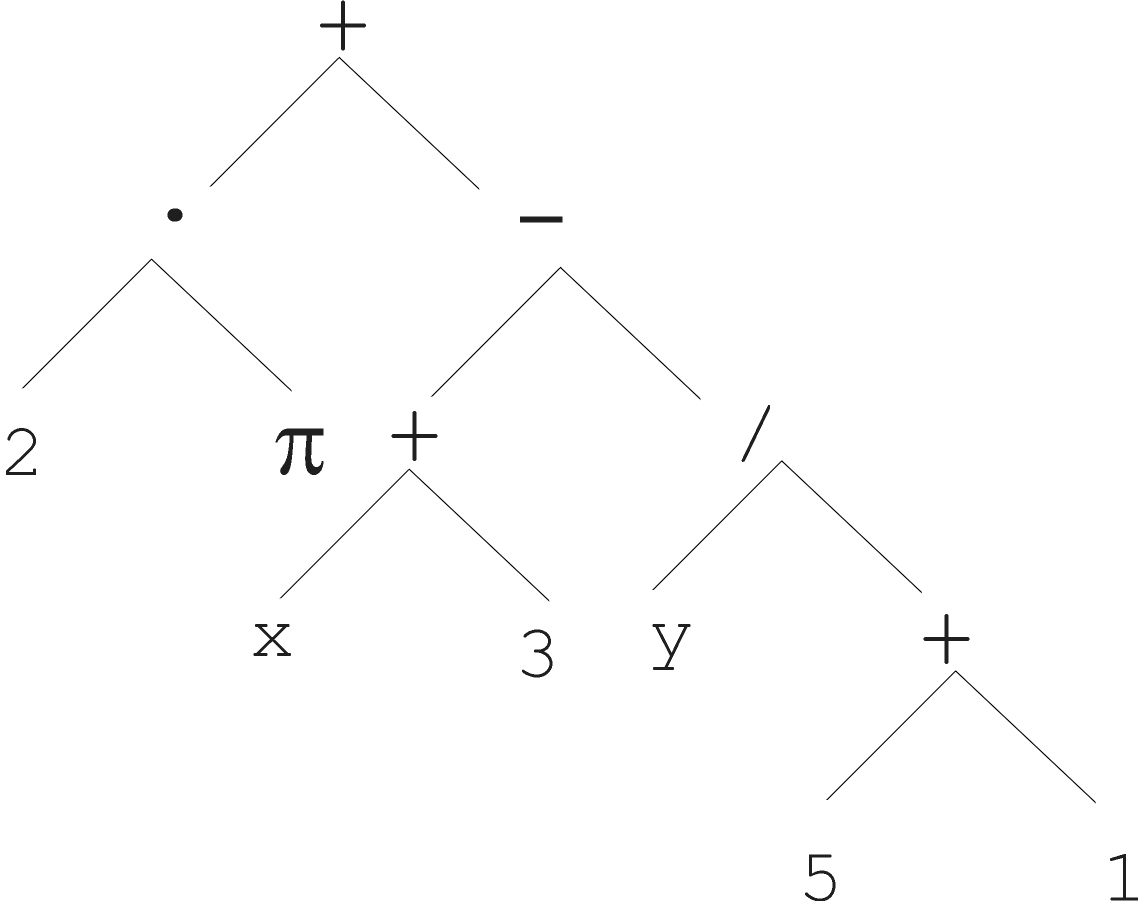
Arithmetic formula:
\(2 \cdot \pi + ((x + 3) - \frac{y}{5+1})\)
And it’s abstract tree:

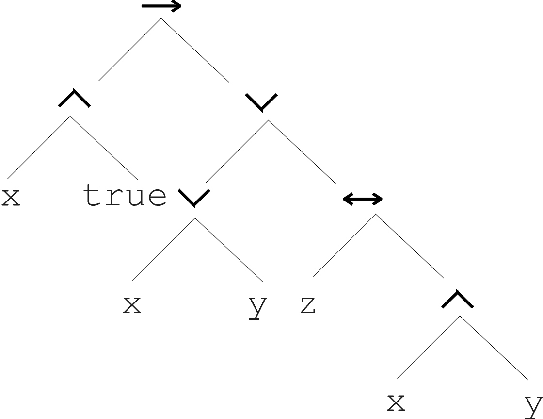
Logical formula:
\((x \land true) \rightarrow ((x \lor y) \lor (z \leftrightarrow (x \land y)))\)
And it’s abstract tree:

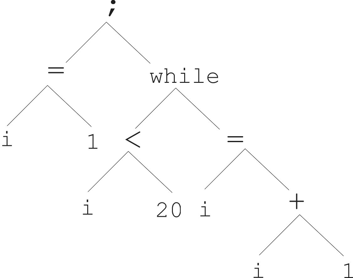
Program:

i = 1;
while(i < 20){
  i = i +1
}

And it’s abstract tree:

1.7.2 Complications of trees

Genetic programming (GP) employs tree representations.
These representations require different methods than before.

1.7.2.1 Non-linear

In GA, ES, and EP, chromosomes are linear structures.
These included bit strings, integer string, real-valued vectors, permutations, etc.
Tree chromosomes in GP are non-linear structures.

1.7.2.2 Variably sized

In GA, ES, and EP, the size of the chromosomes is fixed.
These included various strings of equal length.
Tree chromosomes in GP may vary in depth and width.

1.7.3 Formalization

Representing individuals involves defining the syntax of the trees.
The syntax of the symbolic expressions (s-expressions) represents trees.
Defining a function set and a terminal set.
Allow elements of the terminal set as leaves.
Allow symbols from the function set as internal nodes.

For example:
\(2 \cdot \pi + ((x + 3) - \frac{y}{5+1})\)

Function set {+, −, ·, /}
Terminal set IR ∪ {x, y}

Two general parts are often omitted:
1. Specify the arity for each function in the set.
2. Define correct expressions (trees) on the function and terminal set.

Those parts follow now:
All elements of the terminal set T are correct expressions.
If \(f \in F\) is a function symbol,
with arity n,
and if each of \(e_1, ..., e_n\) is a correct expression, then so is \(f(e_1, ..., e_n)\).
There are no other forms of correct expressions.

To summarize:

• Symbolic expressions can be defined by:
  • Terminal set T
  • Function set F (with the arities of function symbols)
• Adopting the following general recursive definition:

Every \(t \in T\) is a correct expression.
If the following are correct expressions:
\(f \in F\),
\(arity(f)=n\), and
\(e_1, ..., e_n\)
then, \(f(e_1, ..., e_n)\) is a correct expression.
There are no other forms of correct expressions.

1.7.4 Typing

In the original standard GP, expressions are not typed.
In the above definition, we do not distinguish different types of expressions.
Each function symbol in the example can take any expression as argument.
This feature is known as the closure property.
Formally, any \(f \in F\) can take any \(g \in F\) as an argument.

In practice, function symbols and terminal symbols are often typed.
Typed symbols impose extra syntactic requirements.
A problem might require both arithmetic and logical function symbols.
For example, typing enables (N = 2) ∧ (S > 80.000)) as a correct expression.
In this latter example, it is necessary to enforce another rule:
Arithmetic (logical) function symbols only have arithmetic (logical) arguments.
For example, this excludes N ∧ 80.000 as a correct expression.
Strongly typed genetic programming (STGP) addresses this issue.

1.7.5 Mutation

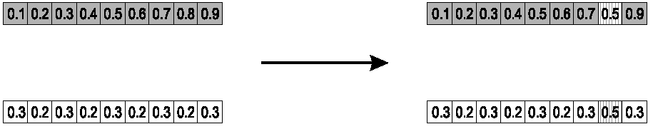
The most common implementation of tree-based mutation works as follows:

Select a node at random from the tree.
Replace the sub-tree starting there with a randomly generated tree.
This newly created sub-tree is usually generated the same way as in the initial population.
It is also subject to conditions on maximum depth and width.
The image illustrates how the parse tree example above (left) is mutated into one standing for \(2 \cdot \pi + ((x + 3) - y)\).
As one goes down through a tree there are potentially more nodes at any given depth.

Size
The size, or tree depth, of the child can exceed that of the parent tree.
In this regard, mutation within GP differs from mutation in other EC dialects.

Tree-based mutation is illustrated here:

The node designated by a circle in the tree on the left is selected for mutation.
The sub-tree staring at that node is replaced by a randomly generated tree, which is a leaf here.

Tree-based mutation has two parameters:
First, the probability of choosing mutation itself, instead of, or in addition to, recombination, p_m
Second, the probability of choosing an internal point within the parent as the root of the sub-tree to be replaced.

It is remarkable that Koza’s classic book on GP from 1992 advises users to set the mutation rate at 0.
This suggests GP works without mutation!
More recently Banzhaf et al. recommended 5%.
In giving mutation such a limited role, GP differs from other EA streams.
The generally shared view is that crossover has a large shuffling effect, acting in some sense, as a macro-mutation operator.
The current GP practice uses low, but positive, mutation frequencies,
even though some studies indicate that the common wisdom favoring an (almost) pure crossover approach might be misleading.

1.7.6 Recombination

Tree-based recombination creates offspring by swapping genetic material among the selected parents.
It is a binary operator, taking two parent trees, to create two child trees.
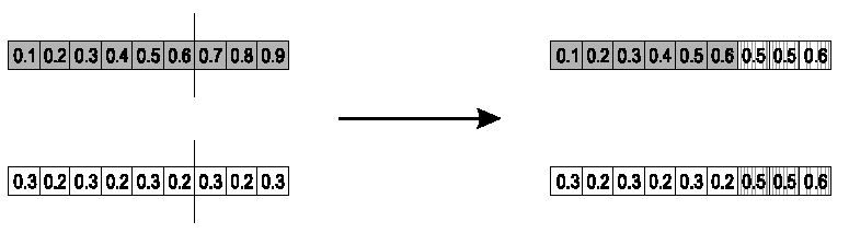
The most common implementation is sub-tree crossover.
Start at two randomly selected nodes in the given parents.
Each node is a sub-tree.
Interchanging those two sub-trees.

Size
Like in mutation, size (tree depth) of the children can exceed that of the parent trees.
In this regard, recombination within GP differs from recombination in other EC dialects.

Tree-based recombination has two parameters:
First, the probability of choosing recombination at the junction with mutation, p_c
Second, the probability of choosing internal nodes as crossover points

Tree-based crossover is illustrated here:

The nodes designated by a circle in the parent trees are selected to serve as crossover points.
The sub-trees staring at those nodes are swapped, resulting in two new trees, which are the children.

We’ll cover this representation more with genetic programming, near the end of this class:
18-GeneticProgramming.html

Next: 05-FitnessSelection.html