Two fundamental forces form the basis of evolutionary systems:
Previous: 04-RepresentMutateRecombine.html
Two fundamental forces form the basis of evolutionary systems:
variation and selection.
These opposing forces are both necessary.
Maintaining diversity is important,
but not sufficient.
Selection for more fit individuals is important,
but not sufficient.
Each is one side, of a dual process.
https://en.wikipedia.org/wiki/Selection_(genetic_algorithm)
Selection for fitness is the second fundamental force driving
evolution.
By selection for fitness, we mean meritocratically determined,
differential success in survival and reproduction.
We will cover:
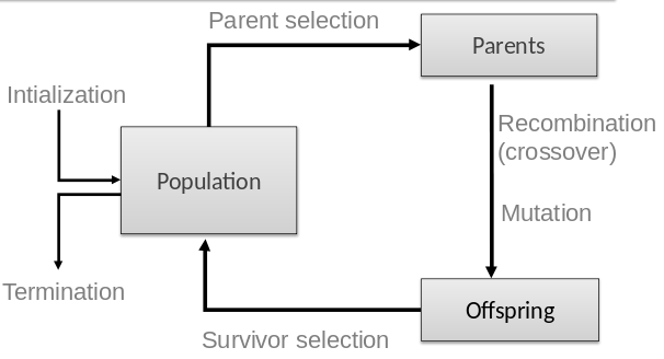
Two different population management models exist:
In each generation we begin with a population of size μ,
from which a mating pool of parents is selected.
Every member of the pool is derived from something in the
population.
The proportions from each parents will probably differ,
with usually more copies of the ‘better’ parents.
Next, λ offspring are created from the mating pool,
through the application of variation operators.
Offspring are evaluated by the fitness function.
From the offspring, select μ individuals as then next generation.
In the model typically used within the Simple Genetic
Algorithm,
the population, mating pool, and offspring are all the same size,
so that each generation is replaced by all of its offspring.
This restriction to use all offspring is not necessary.
For example in the (μ, λ) Evolution Strategy,
typically λ/μ is in the range 5-7.
Create an excess of offspring,
and select only the best fraction.
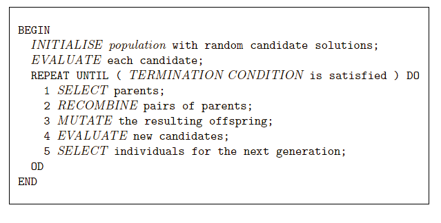
Summary
In the steady-state model,
the entire population is not changed synchronously at once.
λ (< μ) old individuals are replaced by λ new offspring.
The steady-state model has been widely studied and applied.
is the proportion of the population that is replaced,
when after breeding produces more children,
we cull back to μ.
Formally, it is:
λ/μ
For generational, it is often λ/μ = 1.0
We replace all parents with children.
For steady state, it is often, λ = 1/pop_size
We replace 1 (generally bad and/or old) parent with 1 new child.
Summary
Operators responsible for competition in population management,
work on the basis of an individual’s fitness value itself.
Abstract fitness rank is independent of representation.
Selection and replacement operators work independently of the problem
representation.
Fitness-based competition occurs at two points in the evolutionary cycle:
Many mechanisms can be used for either.
We will adopt a convention that:
we are trying to maximize fitness,
and that fitness values are not negative.
We often express problems in terms of an objective function to be
minimized,
For some formulations negative fitness values occur.
We can map these into the desired form by using an appropriate
transformation.
We review several different parent selection mechanisms.
Some of these can be used for survivor selection too.
https://en.wikipedia.org/wiki/Fitness_proportionate_selection
https://en.wikipedia.org/wiki/Selection_(genetic_algorithm)#Roulette_Wheel_Selection
The probability that an individual, i, is selected for mating, depends
on a ratio,
of the individual’s fitness, relative to the population’s fitness.
The sum of the probabilities over the whole population should equal
1.
The selection probability of individual i can be defined as:
\(P_{FPS}(i) = f_i / \sum_{j=1}^{u}
f_j\)
This selection mechanism has been the topic of intensive study.
It is particularly amenable to theoretical analysis.
There are some problems with this selection mechanism:
Initially outstanding individuals can take over the entire population
quickly.
This is known as premature convergence.
It tends to focus the search process.
It decreases the probability the algorithm will thoroughly search,
through the space of possible solutions.
Better solutions may exist.
This phenomenon is often observed in early generations.
To make the problem worse, in early generations,
most randomly created individuals will likely have low fitness.
When fitness values are all very close together,
selective pressure is reduced.
Thus, selection approaches random.
Having a slightly better fitness, is not very ‘useful’ to an
individual.
Later in a run, some convergence has taken place,
and the worst individuals are gone.
Then, it is often observed that the mean population fitness may only
increase very slowly.
FP behaves differently if the fitness function is linearly
transposed.
The table shows three individuals and a fitness function with:
f(A) = 1, f(B) = 4, f(C) = 5
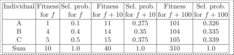
Transposing this fitness function changes the selection
probabilities.
The ordinal linkage of the fitness landscape,
and hence the location of the optimum,
remains the same.
To avoid the second two problems with FPS,
we employ a procedure called windowing.
Fitness differentials are maintained by:
subtracting from the raw fitness f(x) a value βt,
which depends in some way on the recent search history,
and so can change over time or iterations
(hence the superscript t).
It is often not a strict function of time,
but of the population that happens to exist,
at any given time.
One approach subtracts the value of the least-fit member of the current
population,
Pt by setting:
\(\beta^t = min_{y \in p^t}
f(y)\)
We then re-compute the fitness:
\(f'(x) = f(x) - \beta^t\)
What effect does that have?
βt value may fluctuate quite rapidly,
so one alternative is to use a running average,
over the last few generations.
This is like normalizing grades to the best student in the
class.
Normalizing to a max or min is common.
Another well-known approach is sigma scaling.
It incorporates summary information for fitnesses in the
population:
the mean \(\bar{f}\) and
standard deviation \(\sigma_f\)
where c is a constant value,
usually set to 2:
\(f'(x) = max(f(x) - (\bar{f} - c \cdot
\sigma_f), 0)\)
What effect does that have?
Normalization!
https://en.wikipedia.org/wiki/Selection_(genetic_algorithm)#Rank_Selection
Rank-based selection was designed to address previous problems.
It preserves a constant differential selection pressure.
It sorts the population on the basis of fitness.
Selection probabilities map to individuals according to their
rank,
rather than according to their raw fitness.
If we define ranks as decreasing numbers,
then an individual’s rank implies the number of worse solutions in the
population.
Specifically, the best has rank μ-1,
and the worst has rank 0.
In any selection scheme,
we require that the sum over the population of the selection
probabilities must be unity.
The cumulative probability is often thought of as 1.
That the sum not less than 1,
implies that we must select one of the parents.
We must mapping from rank number to selection probability.
The mechanism of mapping can vary.
The simplest concept to map this idea would be:
\(P_{lin-too-simple^{(i)}} =
\frac{i}{\mu}\)
μ is fixed, population size.
i is rank, decreasing.
Observe that:
with high rank (large i), p(i) is high.
05-FitnessSelection/rank_linear_simple.py
#!/usr/bin/python3
"""
This one behaves more like a cumulative probability.
"""

import matplotlib.pyplot as plt

u = 200
ui = range(u)
fitnesses = []
for i in range(u):
    P_i = i / u
    print(f"Fitness of {i}, P_i is {P_i}")
    fitnesses.append(P_i)
plt.plot(ui, fitnesses)
plt.show()
Note: this looks like a cumulative probability
distribution,
which we used before:
03-MetaheuristicParts.html#run-1-cycle
A common real linear ranking schemes is parameterized by a value s (1
< s ≤ 2).
In the case of a generational EA, where μ = λ,
this can be interpreted as:
the expected number of offspring allotted to the fittest
individual.
Since this individual has i (rank) defined as μ − 1,
and the worst has i (rank) is 0,
the selection probability for an individual of rank i is:
\(P_{lin-rank^{(i)}} = \frac{(2-s)}{\mu} +
\frac{2i(s-1)}{\mu(\mu-1)}\)
The first term will be constant for all individuals.
It is there to ensure the probabilities add to one.
Did my bad example above do that?
Since the second term will be zero for the worst individual (with rank i
= 0),
it can be thought of as the ‘baseline’ probability of selecting that
individual.
s just pushes the proportion in a direction of favorable.
s can be meta-optimized.
05-FitnessSelection/rank_linear.py
#!/usr/bin/python3
"""
When s = 1,
this would add up to the cumulative probability of the linear_rank_simple.py
"""

import numpy as np
import matplotlib.pyplot as plt

u = 10
ui = range(u)
s_values = np.arange(1, 2.1, 0.1)
for s in s_values:
    print(f"\nS value of {s}")
    fitnesses = []
    for i in range(u):
        fitness_i = ((2 - s) / u) + ((2 * i) * (s - 1)) / (u * (u - 1))
        fitnesses.append(fitness_i)
        print(f"fitness of {i} is {fitness_i}")
    plt.plot(ui, fitnesses, label=f"{s}")
plt.legend()
plt.show()
Example: FP versus Linear Rank
We show an example of how the selection probabilities differ for
a population of μ = 3 different individuals,
with fitness proportionate versus rank-based selection,
with different values of s.
Parameterized by factor s:
1 < s ≤ 2.
Measures advantage of best individual:
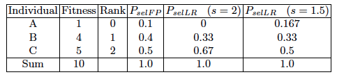
FP is not linear: e.g., 0.5-0.4=0.1 and 0.4-0.1=0.3
LR produces linear differentials between individuals.
When the mapping from rank to selection probabilities is linear,
only limited selection pressure can be applied.
This arises from the assumption that, on average,
an individual of median fitness should have one chance to be
reproduced,
which in turn imposes a maximum value of s = 2.
Given the equation above, letting s > 2,
would require the worst to have a negative selection probability.
Recall: the probabilities are defined to sum to unity.
We may want a higher selection pressure on top individuals.
To put more emphasis on selecting individuals of above-average
fitness,
an exponential ranking scheme is often used.
Since this individual has i (rank) defined as μ − 1,
and the worst has i (rank) is 0,
the selection probability for an individual of rank i is:
e is Euler’s number:
https://en.wikipedia.org/wiki/E_(mathematical_constant)
\(P_{exp-rank^{(i)}} =
\frac{1-e^{-i}}{c}\)
The normalization factor c,
is chosen so that the sum of the probabilities is unity,
i.e., it is a function of the population size.
Linear Ranking is limited in selection pressure.
Exponential Ranking can allocate an average of more than 2 copies to
fittest individual.
We can normalize the constant factor, c, according to
population size.
Finally, from the resulting probability distribution,
we sample the next pool using something like:
roulette wheel, stochastic universal sampling, etc.
These are illustrated in the next section.
05-FitnessSelection/rank_exp.py
#!/usr/bin/python3
"""
Exponential ranking
"""
import numpy as np
import matplotlib.pyplot as plt

# Population size
u = 20
ui = range(u)
# Normalization constant:
c = u - (1 - (1 / np.exp(u))) / (1 - np.exp(-1))
fitnesses = []
for i in range(u):
    e = np.exp(1)
    P_i = (1 - (e**-i)) / c
    print(f"Fitness of {i}, P_i is {P_i}")
    fitnesses.append(P_i)
print(sum(fitnesses))
plt.plot(ui, fitnesses)
plt.show()We attempt to address the problems of FP,
by basing selection probabilities on relative rather than
absolute fitness.
We rank the population according to fitness,
and then base selection probabilities on rank.
The fittest has rank u-1 and worst rank 0.
Computationally, this imposes a sorting overhead on the algorithm.
However, this is usually negligible compared to the fitness evaluation
time!
A probability distribution defines the likelihood of each individual in the population being selected for reproduction.
Recall:
03-MetaheuristicParts.html#run-1-cycle
Where I implement the “marbles in a bucket” algorithm,
which assumes the popuulation size is 100.
We previously covered two schemes for defining a probability
distribution.
Ideally, the mating pool of parents taking part in recombination,
would have exactly the same proportions as this selection probability
distribution.
This would mean that the number of any given individual,
would be given by its selection probability,
multiplied by the size of the mating pool.
In practice this is not possible with a finite sized population.
When we do the multiplications to calculate probabilities,
we typically find that some individuals have an expected number of
copies,
which is non-integer, often less than 1.
Yet, we need to select complete individuals.
The mating pool of parents is sampled from the selection probability
distribution,
but will not in always perfectly reflect it’s proportions.
The simplest way to sample is known as the roulette wheel
algorithm.
By analogy to roulette,
assuming the sizes of the holes reflect the selection
probabilities,
This is like repeatedly throwing one ball onto this spinning
wheel:

In general, the algorithm can be applied to a set of μ parents to select
λ members.
The λ individuals form the mating pool.
We will assume some order over the population (ranking or random) from 1
to μ,
so that we can calculate the cumulative probability
disibutribution,
which is a list of values [a1, a2, …, aµ],
such that:
\(a_i = \sum_1^i P_{sel^{(i)}}\)
where \(P_{sel^{(i)}}\) is defined by
the selection distribution,
derived from either fitness proportionate (FP) or ranking.
Note that this implies aµ = 1.
Recall our example from the simple evolution of x2?
Show that now:
03-MetaheuristicParts.html#run-1-cycle
The important part:
We are given the cumulative probabilily
distribution,
a list of probabilities for each individual.
Roulette wheel algorithm:
BEGIN
    /* Given the cumulative probability distribution, a, */
    /* and assuming we wish to select λ members of the mating pool */
    set current_member = 1;
    WHILE ( current_member ≤ λ ) DO
        Pick a random value, r, uniformly from [0, 1];
        set i = 1;
        WHILE ( a_i < r ) DO
            set i = i + 1;
        OD
        set mating_pool[current_member] = parents[i];
        set current_member = current_member + 1;
    OD
END
Ask:
How many times does the outer while loop execute?
Despite its simplicity,
and logical consistency,
it may not provide representative sample of the distribution.
https://en.wikipedia.org/wiki/Stochastic_universal_sampling
Whenever more than one sample is to be drawn from the
distribution,
for instance, λ for a mating pool,
the use of the stochastic universal sampling (SUS) algorithm is
preferred.
By analogy to roulette,
assuming the sizes of the holes reflect the selection
probabilities,
this is equivalent to making one spin of a wheel with λ equally spaced
arms,
rather than λ spins of a one-armed wheel.

Given the same list of cumulative selection probabilities,
[a1, a2, …, aµ],
it performs λ selections, choosing the mating pool.
Stochastic universal sampling algorithm:
BEGIN
    /* Given the cumulative probability distribution a */
    /* and assuming we wish to select λ members of the mating pool */
    set current_member = i = 1;
    Pick a random value, r, uniformly from [0, 1/λ];
    WHILE ( current_member ≤ λ ) DO
        WHILE ( r ≤ a[i] ) DO
            set mating_pool[current_member] = parents[i];
            set r = r + 1/λ;
            set current_member = current_member + 1;
        OD
        set i = i + 1;
    OD
END
Ask:
How many times does the outer while loop execute?
Since the value of the variable r is initialised in the range [0,
1/λ],
and increases by an amount 1/λ every time a selection is made,
it is guaranteed that the number of copies made of each parent i,
is at least the integer part of \(\lambda
\cdot P_{sel^{(i)}}\),
and is no more than one greater.
Finally, we should note that with minor changes to the code,
SUS can be used to make any number of selections from the parents,
and in the case of making just one selection,
it is the same as the roulette wheel.
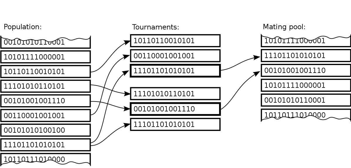
https://en.wikipedia.org/wiki/Tournament_selection
Repeated competitions between k individuals select breeders.
E.g., k=3:
The previous two selection methods,
and the algorithms used to sample from their probability
distributions,
relied on a knowledge of the entire population.
If the population size is very large,
or if the population is distributed in some way (perhaps on a parallel
system),
obtaining this knowledge is either highly time consuming,
or at worst impossible.
https://www.youtube.com/watch?v=YZUNRmwoijw
Both methods assume that fitness is an directly quantifiable
measure,
based on some explicit objective function,
to be optimized in a vacuum.
This assumption may not always be practically true.
Imagine evolving game playing strategies.
We might not be able to quantify the strength of a given individual
(strategy) in isolation.
We may need to compare any two of them,
by simulating a game played by these strategies as opponents.
The success of the strategy is still merely and indicator of the
fitness,
under varied conditions, opponents’ strategies.
https://en.wikipedia.org/wiki/Evolutionary_art
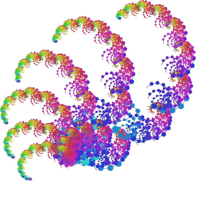
Similar situations occur also in evolutionary art applications.
The fitness function is a human’s judgement.
The user makes a subjective selection,
by comparing individuals representing designs or pieces of art,
rather than using a quantitative measure to assign fitness.
https://en.wikipedia.org/wiki/Evolutionary_music
05-FitnessSelection/Music_Shao2010.pdf
05-FitnessSelection/Music_Loughran2012.pdf
05-FitnessSelection/Music_Loughran2016a.pdf
05-FitnessSelection/Music_Loughran2016b.pdf
05-FitnessSelection/Music_Loughran2017a.pdf
05-FitnessSelection/Music_Loughran2017b.pdf
05-FitnessSelection/Music_Loughran2020.pdf
This problem is not limited to art,
but any problem where the human is the fitness function.
More broadly, it can be considered a sub-field.
For example, ergonomics, advertising, etc.
This is sometimes called:
interactive evolutionary computing,
human-in-the-loop, or
interactive EC.
https://en.wikipedia.org/wiki/Interactive_evolutionary_computation
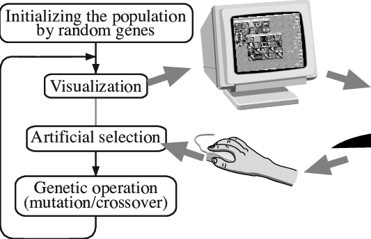
Interactive evolutionary computation (IEC) or aesthetic selection is a
general term for methods of evolutionary computation that use human
evaluation.
Usually human evaluation is necessary when the form of fitness function
is not known (for example, visual appeal or attractiveness;
or the result of optimization should fit a particular user
preference
(for example, taste of coffee or color set of the user interface).
An interactive genetic algorithm (IGA) is defined as a genetic
algorithm that uses human evaluation.
These algorithms belong to a more general category of Interactive
evolutionary computation.
The main application of these techniques include domains where it is
hard or impossible to design a computational fitness function.
For example, evolving images, music, various artistic designs and forms
to fit a user’s aesthetic preferences.
Interactive computation methods can use different representations,
both linear (as in traditional genetic algorithms)
and tree-like ones (as in genetic programming).
Human-based EC is a bit different of a notion:
https://en.wikipedia.org/wiki/Human-based_evolutionary_computation
https://en.wikipedia.org/wiki/Human-based_genetic_algorithm
We can also evolve things for the human, such as a more optimal
keyboard:
https://www.youtube.com/watch?v=EOaPb9wrgDY
Another example of bad keyboards (show this one in class):
https://www.youtube.com/watch?v=188fipF-i5I
No global knowledge of the population,
nor a quantifiable measure of quality.
Instead, it only relies on an ordering relation,
that can compare and rank any two individuals.
It is therefore conceptually simple,
and fast to implement and apply.
The application of tournament selection,
to select λ members of a pool of μ individuals,
works according to the following procedure:
Tournament selection:
BEGIN
    /* Assume we wish to select λ members of a pool of µ individuals */
    set current_member = 1;
    WHILE ( current_member ≤ λ ) DO
        Pick k individuals randomly, with or without replacement;
        Compare these k individuals and select the best of them;
        Denote this individual as i;
        set mating_pool[current member] = i;
        set current_member = current_member + 1;
    OD
ENDTournament selection evaluates relative fitness,
rather than absolute fitness.
Thus, it shares properties with previous ranking schemes.
Both demonstrate invariance to translation and transposition of the
fitness function.
Four factors impact the probability of selecting an individual in a
tournament:
Individual rank in the population.
Tournaments estimate rank,
without directly sorting the whole population.
The larger the tournament size, k,
the greater the chance that it will contain members of above-average
fitness,
and the lesser the chance that it will consist entirely of low-fitness
members.
As k is increases,
the probability of selecting a high-fitness member increases,
and that of selecting a low-fitness member decreases.
Increasing k increases the selection pressure.
p defines the probability that the most fit member of the tournament
is selected.
Deterministic tournament outcomes define p = 1.
Stochastic tournament outcomes permit p < 1.
Since stochasticity makes it more likely that a less-fit member is
selected,
decreasing p will decrease the selection pressure.
Whether individuals are chosen with, or without replacement,
to participate in the tournament.
This replacement choice is before competing.
For simplicity of this sub-analysis,
we temporarily assume deterministic tournaments:
Without replacement:
The k-1 least-fit members of the population can never be selected,
since the other member of the tournament will be fitter.
With replacement:
All tournament candidates could randomly be copies of the worst
member.
This, it is possible for the least-fit member of a population to be
selected.
With a low probability, 1/μk > 0,
Timing similarities
For binary (k = 2) tournaments with parameter p (determinism of
outcome),
the expected time for a single individual of high fitness to take over
the population,
is roughly the same as that for linear ranking with s = 2p.
Weakness similarities
Since λ tournaments are required to produce λ selections,
it suffers from similar problems as the roulette wheel algorithm.
Specifically, with low n,
the observed outcomes can differ greatly,
from the theoretical probability distribution,
Despite these drawbacks,
tournament selection is a widely used selection operator in some EC
dialects,
(in particular, Genetic Algorithms).
It is simple.
Selection pressure is easy to control,
by varying the tournament size, k.
And, most importantly, it can handle implicit value.
Summary
(i.e., entirely random parental selection)
In some dialects of EC,
it is common to select each individual for breeding with the same
probability.
This might appear to suggest that there is no selection pressure in the
algorithm,
which would indeed be true,
if this was not coupled with a strong fitness-based survivor selection
mechanism.
In Evolutionary Programming,
usually there is no recombination,
only mutation,
and parent selection is deterministic.
Each parent produces exactly one child by mutation.
Evolution Strategies usually randomly select parents for
mating,
i.e.,
for each 1 ≤ i ≤ μ ,
we have:
Puniform(i) = 1/μ.
Summary
Parents are selected by uniform random distribution,
whenever an operator needs one/some.
Uniform parent selection is unbiased.
Every individual has the same probability to be selected.
When working with extremely large populations,
over-selection can be used.
In many cases,
it may be desirable to work with extremely large populations.
For example, implementing EAs using graphics cards (GPUs),
which offer similar speed-up to clusters or supercomputers,
but at much lower cost.
However, achieving the maximum potential speed-up,
typically depends on having a large population on each processing
node.
If the potential search space is enormous,
it might be a good idea to use a large population,
to avoid ‘missing’ promising regions in the initial random
generation,
and thereafter to maintain the diversity needed to support
exploration.
GP often employs population sizes of several thousands to
millions.
A method called over-selection can be used for population sizes of 1000
and above.
The population is first ranked by fitness,
and then divided into two groups,
the top x% in one,
and the remaining (100 − x)% in the other.
For example, with x at 80,
around 80% of the selection operations choose from the first
group,
and around 20% from the second.
Koza defines some “rule of thumb” values for x,
depending on the population size, show below.
Proportion of ranked population in fitter sub-population,
from which majority of parents are selected:
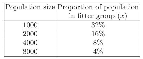
As can be seen,
the number of individuals from which the majority of parents are
chosen,
stays constant,
i.e., the selection pressure increases dramatically for larger
populations.
This step in the main evolutionary cycle is also called
replacement.
Survivor selection mechanisms take set of μ parents and
λ offspring,
and choose a set of μ individuals for the next generation.
In principle, any of the mechanisms introduced for parent
selection,
could be also used for selecting survivors.
Historically, different selection strategies were employed for
survival.
They can be categorized according to whether they discriminate on
either:
1. the age of an individual
2. the fitness of an individual
Each individual exists in the population for the same number of EA
iterations.
Fitness of individuals is not taken into account for replacement.
Copies of highly-fit individuals might still persist in the
population.
However, they would have to be chosen at least once in the parental
selection phase,
and the resulting offspring would have to survive recombination and
mutation stages,
and they would have to escape the recombination and mutation stages
un-modified…
This is quite unlikely, but possible.
Since fitness is not taken into account,
the mean fitness, and even best fitness, of any given generation,
may be lower than that of its predecessor.
While slightly counter-intuitive,
this is the nature of exploration.
Such curiosity may escape a local optimum.
To increase average fitness over time, we must:
have sufficient selection pressure when selecting parents for the mating
pool, and
use variation operators that are not too disruptive.
Age-based replacement is often used in the classic “Genetic Algorithm” methods.
Generational implementations
use the same number of offspring and parents, (μ = λ).
Thus, each individual exists for just one cycle.
The parents are simply discarded,
to be replaced by the entire set of offspring.
This is the generational model we discussed before.
Steady-state implementations
define overlapping populations (λ < μ)
In each cycle, λ new offspring are created,
and inserted in the population.
The parent(s) that produced the offspring is discarded.
The strategy takes the form of a first-in-first-out (FIFO) queue.
Random steady-state versions
For steady-state GAs,
an alternative method to discarding the λ breeding parent(s),
is to randomly select λ parent(s) for replacement.
This probabilistic strategy has the same mean effect.
With λ=1, on average individuals live for μ iterations.
Some work has shown higher variance in performance than a comparable
generational GA.
The random strategy is more likely to lose the best member of the
population.
The random replacement strategy is not recommended.
Fitness selection rules choose individuals for survival.
The fittest of μ parents + λ offspring survive into the next
generation.
A wide number of strategies based on fitness have been proposed.
Some also take age into account.
Replace the worst λ members of the existing μ population.
This can lead to very rapid improvements in the mean population
fitness.
That is not always good.
It can also lead to premature convergence.
The population tends to rapidly focus on the fittest member currently
present.
Thus, it is commonly used in conjunction with large populations,
and/or a “no duplicates” policy.
https://en.wikipedia.org/wiki/Selection_(genetic_algorithm)#Elitism_Selection
Age-based and stochastic fitness-based replacement schemes can discard
fit members.
Elitism prevents the loss of the current fittest member of the
population.
The current fittest member is always kept in the population.
If the fittest current member would be replaced,
and none of the new offspring has equal or better fitness,
then the best is kept,
and one of the offspring is discarded.
https://en.wikipedia.org/wiki/Round-robin_tournament
A round-robin tournament (or all-play-all tournament),
is a competition in which each contestant meets every other
participant,
usually in turn.
This mechanism was introduced within Evolutionary Programming,
where it is applied to choose μ survivors.
In principle, it can also be used to select λ parents from a given
population of μ.
The method works by holding pairwise tournament competitions in
round-robin format.
Each individual is evaluated against q others,
that are randomly chosen from the merged parent and offspring
populations.
For each comparison, a “win” is assigned if the individual is better
than its opponent.
After finishing all tournaments,
the μ individuals with the greatest number of wins are selected.
Often, q = 10 is used in Evolutionary Programming.
This stochastic variant of inclusion in the tournament allows for
less-fit solutions to be selected,
if they had a lucky draw of opponents.
As the value of q increases,
this chance becomes more and unlikely,
until in the limit it becomes deterministic μ + μ.
Offspring and parents are merged,
and ranked according to (estimated) fitness,
then the top μ are kept to form the next generation.
This strategy can be seen as a generalization of the replace-worst
method (μ > λ),
and the round-robin tournament used in Evolutionary Programming where (μ
= λ).
In Evolution Strategies,
λ > μ is often used with a great offspring surplus,
(typically λ/μ ≈ 5-7).
This induces a large selection pressure.
This method works on a mixture of age and fitness.
Typically, λ > μ children are created from a population of μ
parents.
The age component dictates that all the parents are discarded,
so no individual is directly kept for more than one generation
The fitness component ranks λ offspring according to fitness,
and the best μ form the next generation.
The (μ, λ) strategy is often used in Evolution Strategies.
In Evolution Strategies, (μ, λ) selection, is generally preferred
over (μ + λ) selection for the following reasons:
The (μ, λ) discards all parents and is therefore in principle able to
leave (small) local optima.
This may be advantageous in a multimodal search space with many local
optima.
If the fitness function is not fixed,
but changes in time,
the (μ+λ) selection preserves outdated solutions,
so it may not follow a moving optimum well.
The (μ + λ) selection hinders the self-adaptation mechanism used to
adapt strategy parameters (upcoming later).
We have referred informally to the notion of selection
pressure.
As selection pressure increases,
fitter solutions are more proportionately likely to be selected,
and less-fit solutions are proportionately less likely.
We can formalize and quantify this.
The takeover time, τ∗, can be defined for a given selection
mechanism.
The number of generations it takes from one copy,
until the application of selection homogenously fills the population
with that copy.
Some work has shown that:
τ∗ = ln λ / ln(λ/μ)
For a typical evolution strategy,
with μ = 15 and λ = 100,
this results in τ∗ ≈ 2.
For fitness-proportional (FP) selection in a genetic algorithm it
is:
τ∗ = λ ln λ,
resulting in τ∗ = 460 for population size λ = 100.
Other considered solutions such as a a ‘Diversity Indicator’.
One called ‘Expected Loss of Diversity’ is the expected change in the
number of diverse solutions after μ selection events;
“Selection Intensity” is the expected relative increase in mean
population fitness after applying a selection operator.
https://en.wikipedia.org/wiki/Multimodal_distribution
Most interesting problems have more than one locally optimal
solution.
In statistics, a multimodal distribution is a probability distribution
with more than one mode.
These appear as distinct peaks (local maxima) in the probability density
function:
One gene:
Two genes:
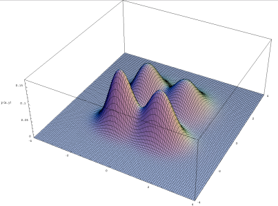
n-genes:
To visualize this, you need to do dimensionality reduction.
But, it still works regardless.
We introduced the concept of local optima.
Effective search relies on the preservation of sufficient
diversity,
to allow both:
exploitation of learned information,
by investigating regions containing high fitness solutions
discovered,
and exploration, in order to uncover new high-fitness regions.
Multimodality is a typical feature of the type of problems for which
EAs are often employed.
One goal is to locate the global optimum, in spite of local optima.
An alternative may be to identify a number of high-fitness
solutions,
corresponding to various local optima.
The latter situation can often arise,
for example, when the fitness function used by the EA does not
completely specify the underlying problem.
An example of this might be in the design of a new widget,
where the parameters of the fitness function may change during the
design process,
as progressively more refined and detailed models are used over
time,
as decisions are made, such as the choice of materials, etc.
In this situation, it is valuable to be able to examine a number of
possible options,
first to permit room for human aesthetic judgments, and
second because it is probably desirable to use solutions from niches
with broader peaks,
rather than from a sharp peak.
This is because the latter may be over-fitted (that is, overly
specialized) to the current fitness function,
and may not be as good once the fitness function is refined.
The population-based nature of EAs excels at identifying multiple optima.
In practice, the finite population size,
when coupled with recombination between any parents
(known as panmictic mixing),
leads to the phenomenon known as genetic drift,
and eventual convergence around one optimum.
The reasons for this can easily be seen:
imagine that we have two equally fit niches,
and a population of 100 individuals,
originally equally divided between them.
Eventually, because of the random effects in selection,
it is likely that we will obtain a parent population,
consisting of 49 of one sort and 51 of the other.
Ignoring the effects of recombination and mutation,
in the next generation the probabilities of selecting individuals from
the two niches are now 0.49 and 0.51 respectively,
i.e., we are increasingly likely to select individuals from the second
niche.
This effect increases as the two sub-populations become unbalanced,
until eventually we end up with only one niche represented in the
population.
Summary
Finite population with global mixing and selection,
eventually convergence around one optimum.
Why?
Often might want to identify several possible peaks.
Sub-optimum mean can still be more attractive,
if we have a number of local optima.
Discussion question:
What is diversity?
Can you attempt a structured or formal definition of diversity?
In a population of solutions, we rely on an assumption:
there can be too much and too little diversity.
Why might that assumption exist in EC?
Review basics of diversity informatics
../../Bioinformatics/Content.html
Lecture 07 diversity informatics:
git clone https://gitlab.com/bio-data/sequence-informatics.git
Unpack this some in lecture.
It is useful to clarify exactly what we mean by “diversity” and
“space”.
Just as biological evolution takes place on a geographic surface,
but can also be considered to occur on an adaptive landscape,
so we can define a number of spaces within which the evolutionary
algorithms operate:
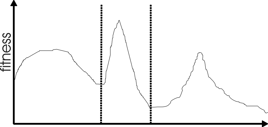
This is the end result:
a search space whose structure is based on distance metrics between
solutions.
The neighborhood structure in this space,
may bear little relationship to that in the genotype space,
according to the complexity of the representation–solution mapping.
We may perceive the set of representable solutions as a genotype
space,
and define some distance metrics.
This can be a natural distance metrics in that space
(e.g., the Manhattan distance, hamming distance)
or based on some fundamental move operator.
Typical move operators include a single bit-flip for binary
spaces,
a single inversion for adjacency-based permutation problems,
and a single swap for order-based permutations problems.
See bioinformatics lecture above.
This is the equivalent of the geographical space,
on which life on Earth has evolved.
Effectively we are considering that the working memory of the EA,
that is, the population of candidate solutions, can be structured in
some way.
This spatial structure could be either a conceptual division, or
real:
for example,
an isolated breeding population might be split over a number of
processors or cores.
A number of mechanisms have been proposed to aid the use of EAs on
multimodal problems.
These can be broadly separated into two camps:
explicit approaches,
in which specific changes are made to operators in order to preserve
diversity, and
implicit approaches,
in which a framework is used that permits,
but does not guarantee,
the preservation of diverse solutions.
Explicit approaches to diversity maintenance,
based on measures of either:
genotype or phenotypic space.
Includes: Fitness Sharing, Crowding, and Speciation,
These work by affecting the probability distributions used by
selection.
Implicit approaches to diversity maintenance,
based on the concept of algorithmic space.
Include Island Model EAs, and Cellular EAs.
Fitness sharing, Crowding, Speciation all shape the probability of selection.
This scheme is based upon the idea that,
the number of individuals within a given niche is controlled,
by sharing their fitness, immediately prior to selection,
in an attempt to allocate individuals to niches,
in proportion to the niche fitness.
In practice, the scheme considers each possible pairing,
of individuals i and j within the population (including i with
itself),
and calculates a distance d(i, j) between them according to some
distance metric
(phenotypic is preferred if possible, else genotypic,
e.g., Hamming distance for binary representations).
The fitness F of each individual i is then adjusted,
according to the number of individuals falling within some pre-specified
distance,
σshare using a power-law distribution:
\(F'(i) = \frac{F(i)}{\sum_j
sh(d(i,j))}\)
where the sharing function sh(d) is a function of the distance d, given
by
\(sh(d) = \left\{ \begin{array}{cc} 1 -
(d/\sigma_{share})^\alpha & if d \leq \sigma_{share}, \\ 0 &
otherwise. \\ \end{array} \right\}\)
The constant value α determines the shape of the sharing function:
for α=1 the function is linear, but for values greater than this,
the effect of similar individuals, in reducing a solution’s
fitness,
falls off more rapidly, with increasing distance.
The value of the share radius σshare decides both:
how many niches can be maintained, and
the granularity with which different niches can be discriminated.
Some suggest that a default value in the range 5-10 should be
used.
Fitness proportionate selection is assumed for the fitness-sharing
method.
There exists a stable distribution of solutions among the niches,
when solutions from each peak have the same effective fitness F’.
Since the niche fitness Fk’ = Fk / nk
,
in this stable distribution each niche k,
contains a number of solutions nk
proportional to the niche fitness Fk1 .
This point is illustrated in below.
Studies have indicated that the use of alternative selection
methods,
does not lead to the formation and preservation of stable
sub-populations in niches.
Summary
Restricts the number of individuals within a given niche by “sharing”
their fitness,
so as to allocate individuals to niches in proportion to the niche
fitness.
Need to set the size of the niche \(\sigma_{share}\),
in either genotype or phenotype space
Run EA as normal but after each generation set.
Note:
if we used sh(d) = 1 for d < \(\sigma_{share}\)
then the sum that reduces the fitness would simply count the number of
neighbors,
i.e., individuals closer than \(\sigma_{share}\)
This creates an advantage of being alone in the neighborhood
Using 1 – d / \(\sigma_{share}\)
instead of 1 implies that we count distant neighbors less
The crowding algorithm was first suggested as a way of preserving
diversity,
by ensuring that new individuals replaced similar members of the
population.
The original scheme worked in a steady-state setting
(the number of new individuals generated in each step was 20% of the
population size).
When a new offspring is inserted into the population,
a number 2 of members of the parent population are chosen at
random,
and then the offspring replaces the most similar of those parents.
A number of problems were found with this approach,
and others have suggested an improvement called deterministic
crowding.
This algorithm relies on the fact that offspring are likely to be
similar to their parents as follows:
1. The parent population is randomly paired.
2. Each pair produces two offspring via recombination.
3. These offspring are mutated and then evaluated.
4. The four pairwise distances between offspring and parents are
calculated.
5. Each offspring then competes for survival in a tournament with one
parent,
so that the inter-competition distances are minimized.
In other words,
denoting the parents as p,
the offspring as o,
and using the subscript to indicate tournament pairing,
d(p1, o1) + d(p2, o2) < d(p1, o2) + d(p2, o1).
The net result of all this is that offspring tend to compete for
survival with the most similar parent,
so sub-populations are preserved in niches but their size does not
depend on fitness;
rather it is equally distributed amongs the peaks available.
The image illustrates this point in comparison with the distribution
achieved under crowding.
Summary
Attempts to distribute individuals evenly among niches.
Relies on the assumption that offspring will tend to be close to
parents.
Eses a distance metric in ph/genotype space.
Randomly shuffle and pair parents, produce 2 offspring.
Set up the parent vs. child tournaments such that the intertournament
distances are minimal.
That is, number the two p’s (parents) and the two o’s (offspring) such
that
d(p1, o1) + d(p2, o2) <
d(p1, o2) + d(p2, o1)
and let o1 compete with p1 and o2
compete with p2
Fitness sharing (top)
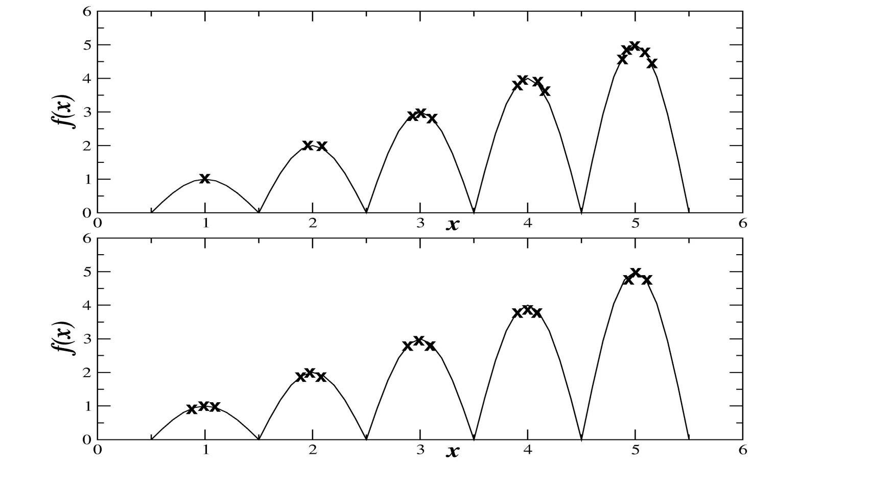
Crowding (bottom)
Which seems like it produces “more diversity”?
The automatic speciation approach imposes mating restrictions based
on some aspect of the candidate solutions (or their genotypes) defining
them as belonging to different species.
The population contains multiple species,
and during parent selection for recombination individuals will only mate
with others from the same (or similar) species.
The biological analogy becomes particularly clear when we note that some
authors refer to the aspect controlling reproductive opportunities as an
individual’s “plumage”.
A number of schemes have been proposed to implement speciation,
which can be divided into two main approaches.
In the first speciation is based on the solution (or its
representation),
e.g., Deb’s phenotype (genotype)-restricted mating.
The alternative approach is to add some elements such as tags to the
genotype that code for the individual’s species,
rather than representing part of the solution.
Many of these ideas were previously suggested by other authors.
These are usually randomly initialized and subject to recombination and
mutation.
Common to both approaches is the idea that once an individual has been
selected to be a parent,
then the choice of mate involves the use of a pairwise distance
metric
(in phenotype or genotype space as appropriate),
with potential mates being rejected beyond a certain distance.
Note that in the tag scheme,
there is initially no guarantee that individuals with similar tags will
represent similar solutions,
although after a few generations selection will usually take care of
this problem.
Neither is there any guarantee that different species will contain
different solutions,
although Spears goes some way towards rectifying this by also using the
tags to perform fitness sharing,
and even without this Deb reported improved performance compared to a
standard GA.
Similarly, although the phenotype-based speciation scheme does not
guarantee diversity maintenance,
when used in conjunction with fitness sharing, it was reported to give
better results than fitness sharing on its own.
Summary
Summary
Island models, Cellular EAs employ more arbitrary geographic constraint,
segmenting populations in algorithmic space.
Summary
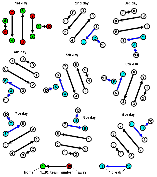
Periodic migration of individual solutions between populations
Run multiple populations in parallel
After a (usually fixed) number of generations (an Epoch),
exchange individuals with neighbors
Repeat until ending criteria met
Partially inspired by parallel/clustered systems
Parameters
Summary
Like a smoothed, continuous island logic, or animals without modern
human travel.
Impose spatial structure (usually grid) in 1 pop
Current
individual
Consider each individual to exist on a point on a (usually rectangular
toroid) grid
Selection (hence recombination) and replacement happen using concept of
a neighborhood a.k.a. deme
Leads to different parts of grid searching different parts of space,
good solutions diffuse across grid over a number of gens
Lexicase selection:
https://www.youtube.com/watch?v=Th6Hx3SJOlk
Novelty search:
05-FitnessSelection/Interesting_and_Novel_greatness.pdf
05-FitnessSelection/Bowren2016.pdf
05-FitnessSelection/Lehman2008.pdf
05-FitnessSelection/Lehman2010a.pdf
05-FitnessSelection/Lehman2010b.pdf
05-FitnessSelection/Lehman2011a.pdf
05-FitnessSelection/Lehman2011b.pdf
05-FitnessSelection/Lehman2011c.pdf
05-FitnessSelection/Lehman2011d.pdf
05-FitnessSelection/Risi2009.pdf
05-FitnessSelection/Risi2010.pdf
05-FitnessSelection/Woolley2013.pdf
05-FitnessSelection/Woolley2014.pdf
This page was mostly about selection,
with hints of fitness functions themselves.