Now, we’ll describe some of the most widely known evolutionary algorithm variants.
Historical EA variants:
More recent versions:
https://en.wikipedia.org/wiki/Genetic_algorithm
http://scholarpedia.org/article/Genetic_algorithms
The genetic algorithm (GA) is the most widely known type of evolutionary
algorithm.
GAs have largely (if mistakenly) been considered as function
optimization methods.
GAs employ:
a binary representation,
fitness proportionate selection,
a low probability of mutation,
an emphasis on genetically inspired recombination,
as a means of generating new candidate solutions.
| Meta-part | Option |
|---|---|
| Representation | Bit-strings |
| Recombination | 1-Point crossover |
| Mutation | Bit flip |
| Parent selection | Fitness proportional, implemented by Roulette Wheel |
| Survivor selection | Generational |
Select parents - for the mating pool.
(size of mating pool = population size)
Shuffle the mating pool.
Apply crossover - for each consecutive pair with probability
pc, otherwise copy parents.
Apply mutation - for each offspring (bit-flip with probability
pm independently for each bit).
Replace the whole population with the resulting offspring.
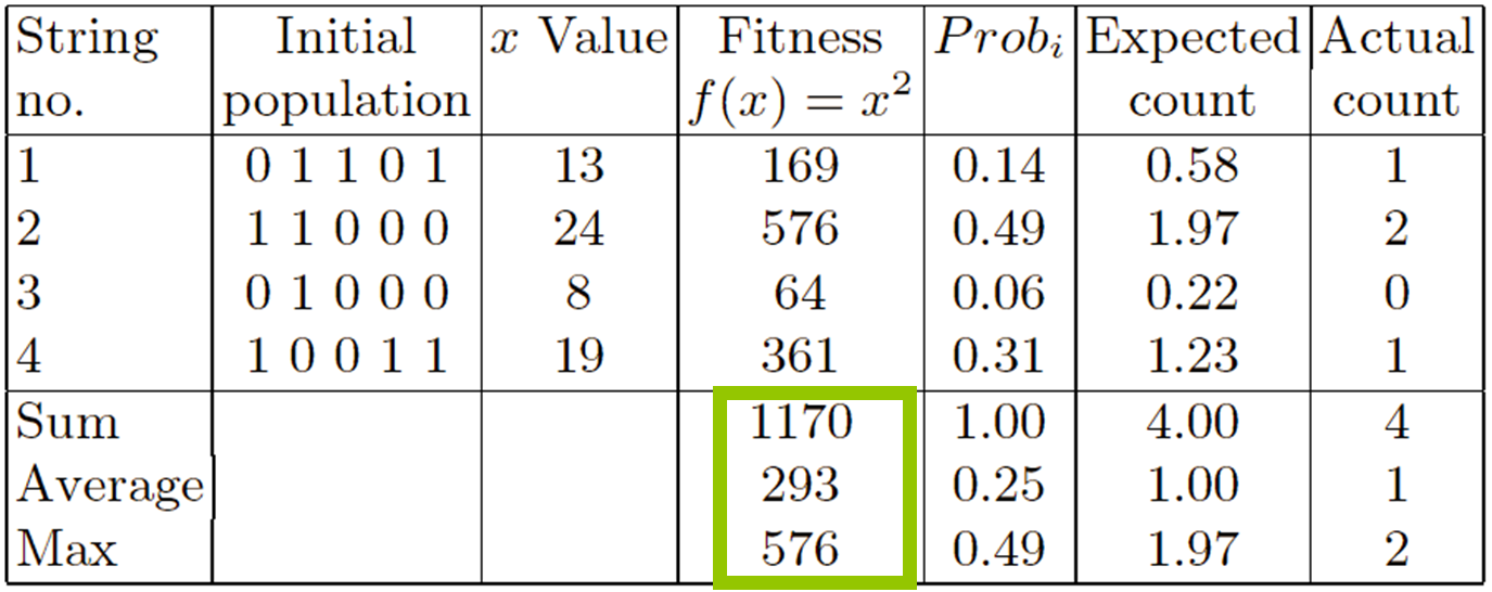
In detail:
GAs traditionally have a fixed work-flow:
given a population of μ individuals,
parent selection fills an intermediary population of μ,
allowing duplicates.
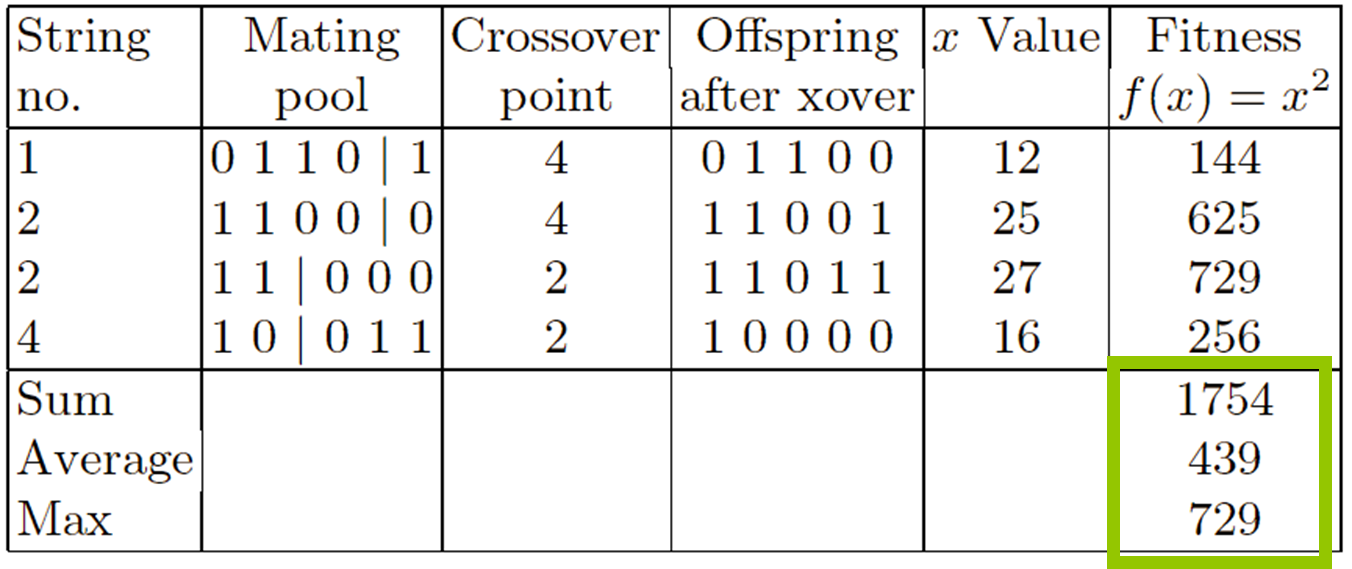
Then the intermediary population is shuffled to create random
pairs,
and crossover is applied to each consecutive pair with probability
pc,
and the children replace the parents immediately.
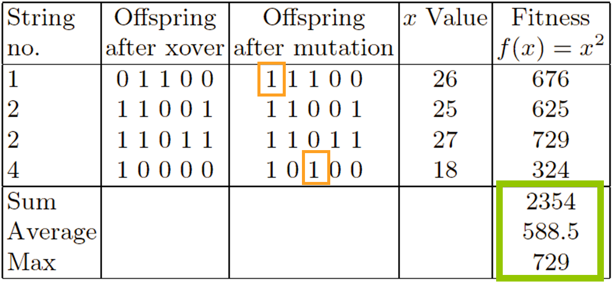
The new intermediary population undergoes mutation individual by
individual,
where each of the l bits in an individual is modified by mutation with
independent probability pm.
The resulting intermediary population forms the next generation
replacing the previous one entirely.
Note that in this new generation there might be pieces,
perhaps complete individuals,
from the previous one that survived crossover and mutation without being
modified,
but the likelihood of this is rather low (depending on the parameters μ,
pc, pm).
We covered this previously.
Has been subject of many (early) studies.
In the early years of the field,
there was significant attention paid to trying to establish suitable
values for GA parameters,
such as the population size, crossover and mutation probabilities.
Recommendations were for mutation rates between 1/l and 1/μ,
crossover probabilities around 0.6-0.8,
and population sizes in the fifties or low hundreds,
although to some extent these values reflect the computing power
available in the 1980s and 1990s.
It has been recognized that there are some flaws in the SGA.
Shows many shortcomings, e.g.,
Representation is too restrictive.
Mutation and crossover operators are only applicable for bit-string and
integer representations.
Selection mechanism is sensitive to converging populations with close
fitness values.
Generational population model can be improved with explicit survivor
selection.
Various features have been added since the first SGA.
Factors such as elitism, and non-generational
models were added to offer faster convergence if needed.
SUS is preferred to roulette wheel
implementation,
and most commonly rank-based selection is used,
implemented via tournament selection for simplicity and
speed.
Studying the biases in the interplay between representation and
one-point crossover led to the development of alternatives,
such as uniform crossover,
and a stream of work through ‘messy-GAs’ and ‘Linkage Learning’,
to Estimation of Distribution Algorithms.
Analysis and experience has recognised the need to use
non-binary representations where more
appropriate.
The problem of how to choose a suitable fixed mutation rate has largely
been solved by adopting the idea of
self-adaptation,
where the rates are encoded as extra genes in an individuals
representation and allowed to evolve.
https://en.wikipedia.org/wiki/Evolution_strategy
http://scholarpedia.org/article/Evolutionary_strategies
This one was actually intended as a numerical optimization
technique.
| Meta-part | Option |
|---|---|
| Representation | Real-valued vectors |
| Recombination | Discrete or intermediary |
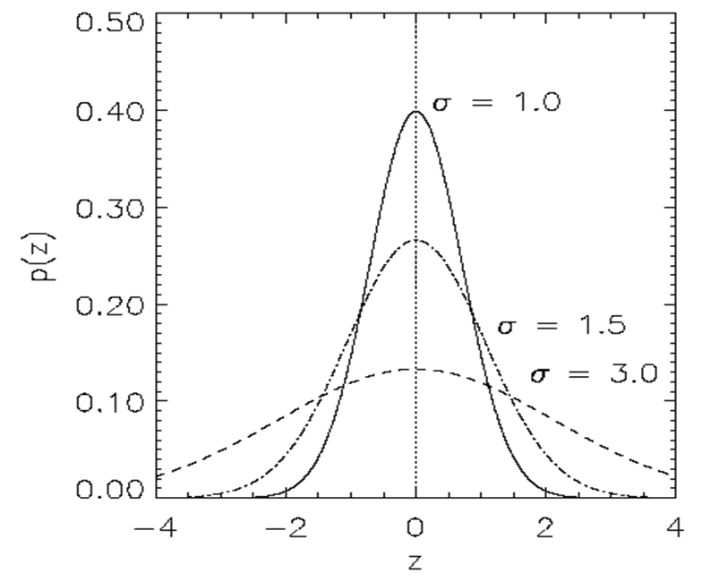
| Mutation | Gaussian perturbation |
| Parent selection | Uniform random |
| Survivor selection | (μ,λ) or (μ+λ) |
Task: minimize f: \({\rm I\!R}^n\) in R
Algorithm: “two-membered ES” using
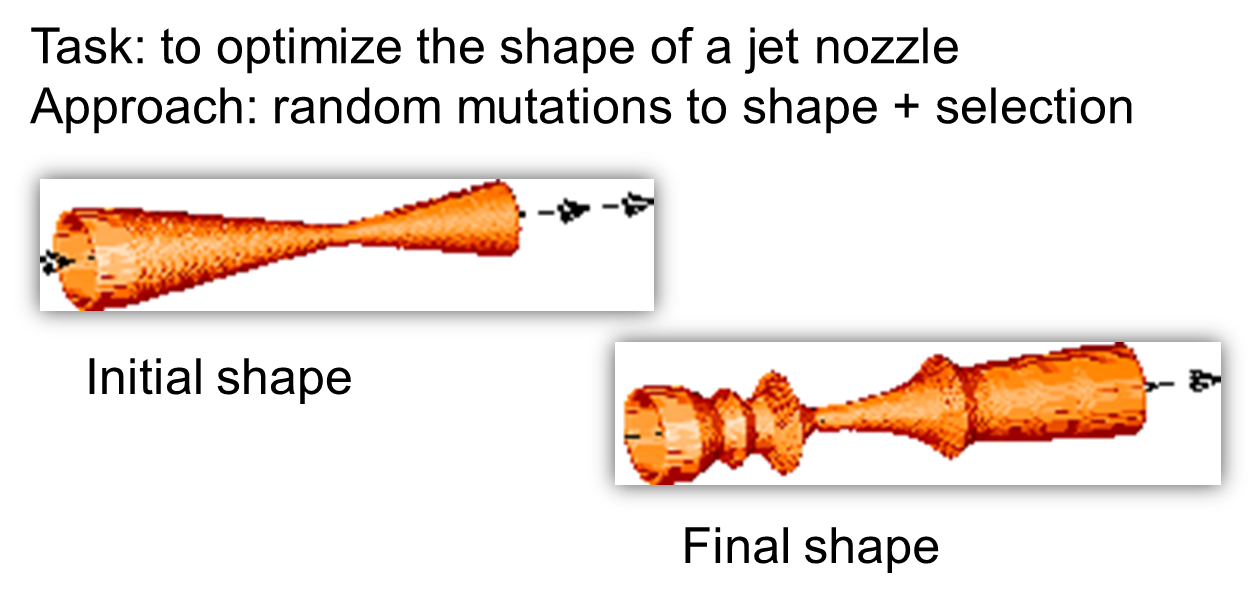
The original nozzle:
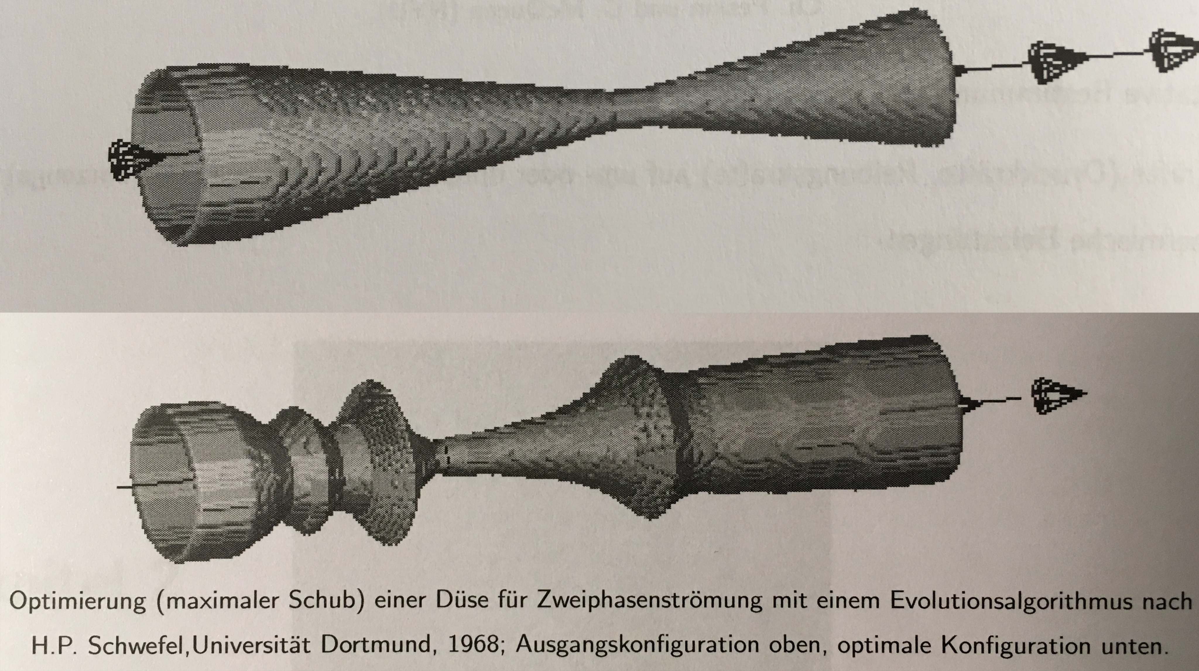
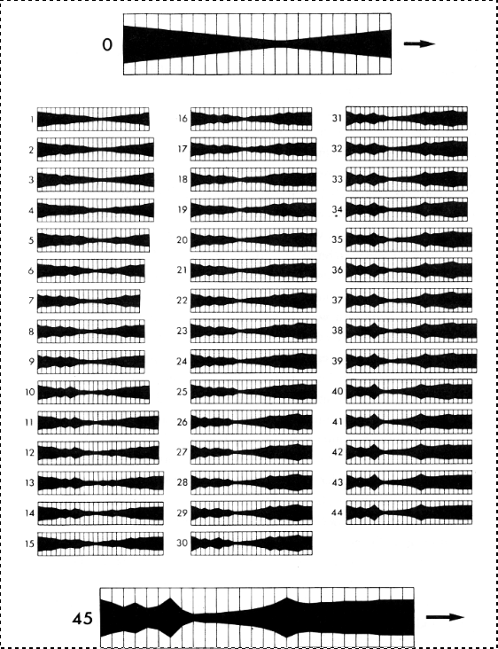
To actually build it:
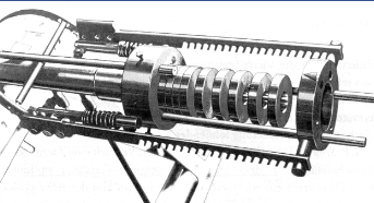
Side note:
Lathing is one of the precursors of precision technologies:
https://www.youtube.com/watch?v=gNRnrn5DE58
ES works with extended chromosomes \(\bar{x}\), \(\bar{p}\),
where \(\bar{x} \in {\rm I\!R}^n\) is a
vector from the domain of the given objective function to be
optimized,
while \(\bar{p}\) carries the algorithm
parameters.
| Two fixed parents | Two parents selected for each i | |
|---|---|---|
| \(z_i = (x_i + y_i)/2\) | Local intermediary | Global intermediary |
| \(z_i\) is \(x_i\) or \(y_i\) chosen randomly | Local discrete | Global discrete |
Parents are selected by uniform random distribution whenever an
operator needs one/some.
Thus, ES parent selection is unbiased.
Every individual has the same probability to be selected.
μ > 1 to carry different strategies.
λ > μ to generate offspring surplus.
(μ,λ)-selection to get rid of mis-adapted σ’s.
Mixing strategy parameters by (intermediary) recombination on them.
Is quite high for ES.
Takeover time \(\tau^*\) is a measure
to quantify the selection pressure.
The number of generations it takes until the application of selection
completely fills the population,
with copies of the best individual.
Goldberg and Deb showed:
For proportional selection in a genetic algorithm the takeover time is
\(\lambda ln(\lambda)\)
Task: to create a color mix yielding a target color (that of a well
known cherry brandy).
Ingredients: water + red, yellow, blue dye
Representation: <w, r, y, b> no self-adaptation!
Values scaled to give a predefined total volume (30 ml).
Mutation: lo / med / hi values of σ used with equal chance.
Selection: (1,8) strategy
Fitness: students effectively making the mix and comparing it with
target color
Termination criterion: student satisfied with mixed color
Solution is found mostly within 20 generations
Accuracy is very good.
https://en.wikipedia.org/wiki/Ackley_function
The Ackley function is widely used for testing optimization
algorithms,
much like an image dataset, or openAI gym, now.
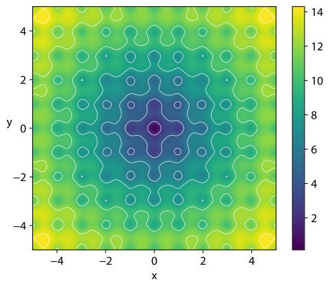
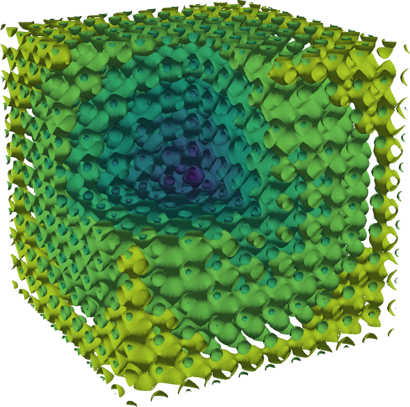
In its two-dimensional form, as shown in the plot above,
it is characterized by a nearly flat outer region,
and a large hole at the centre.
The function poses a risk for optimization algorithms,
particularly hillclimbing algorithms,
to be trapped in one of its many local minima.
https://en.wikipedia.org/wiki/Evolutionary_programming
http://scholarpedia.org/article/Evolutionary_programming
| Meta-part | Option |
|---|---|
| Representation | Real-valued vectors |
| Recombination | None |
| Mutation | Gaussian perturbation |
| Parent selection | Deterministic (each parent one offspring) |
| Survivor selection | Probabilistic (μ+μ) |
EP aimed at achieving intelligence
Intelligence was viewed as adaptive behavior
Prediction of the environment was considered a prerequisite to adaptive
behavior
Thus: capability to predict is key to intelligence
https://en.wikipedia.org/wiki/Finite-state_machine
The original paper:
Fogel, L.J., Owens, A.J., Walsh, M.J.
Artificial Intelligence Through Simulated Evolution
New York: John Wiley, 1966
A discussion of it:
06-PopularVariants/fogel66.pdf
06-PopularVariants/fogel66a.pdf
06-PopularVariants/fogel95.pdf
A population of FSMs is exposed to the environment, that is,
the sequence of symbols that has been observed up to the current
time.
For each parent machine,
as each input symbol is presented to the machine,
the corresponding output symbol is compared with the next input
symbol.
The worth of this prediction is then measured with respect to the payoff
function
(e.g., all-none, squared error).
After the last prediction is made,
a function of the payoff for the sequence of symbols indicates the
fitness of the machine or program
(e.g., average payoff per symbol).
Offspring machines are created by randomly mutating the parents,
and are scored in a similar manner.
Those machines that provide the greatest payoff are retained,
to become parents of the next generation,
and the process iterates.
When new symbols are to be predicted,
the best available machine serves as the basis for making such a
prediction,
and the new observation is added to the available database.
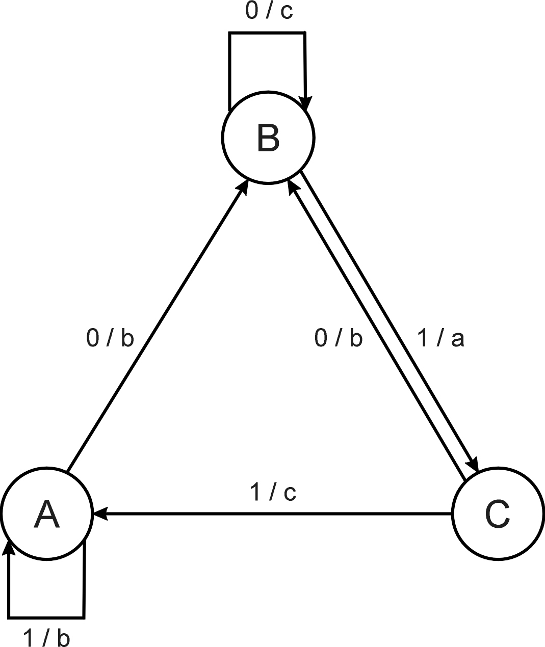
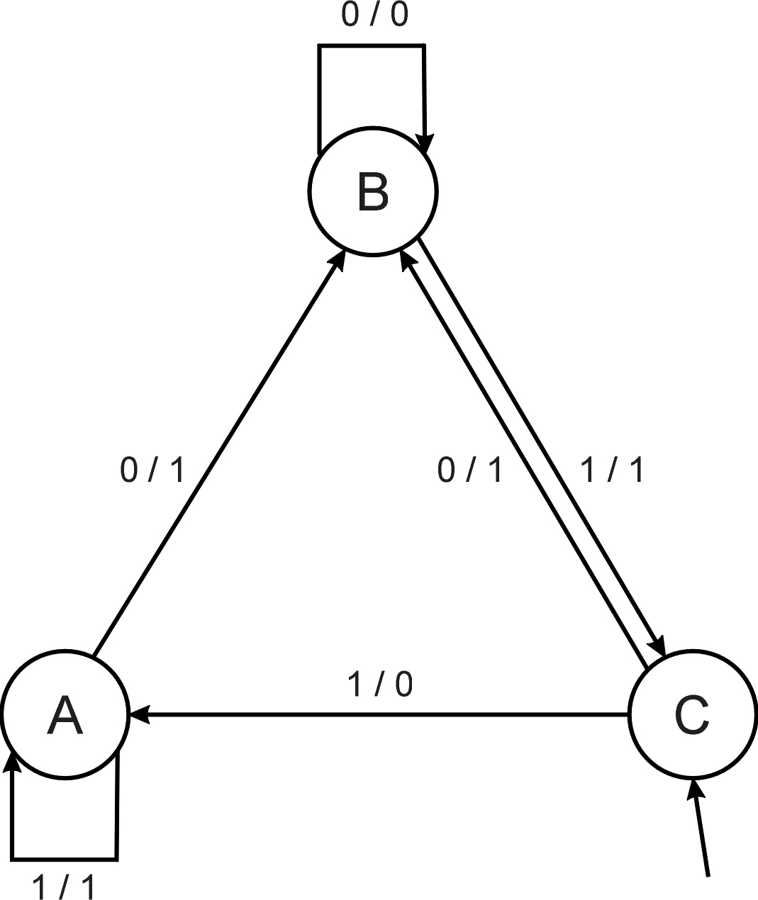
Consider the FSM with:
S = {A, B, C}
I = {0, 1}
O = {a, b, c}
δ given by a diagram (above).
Consider the following FSM
Task: predict next input
Quality (prediction accuracy): % of in(i+1) =
outi
Given initial state C
Input sequence 011101
Leads to output 110111
Quality: 3 out of 5
No predefined representation in general.
Thus, no predefined mutation (must match representation).
Often applies self-adaptation of mutation parameters.
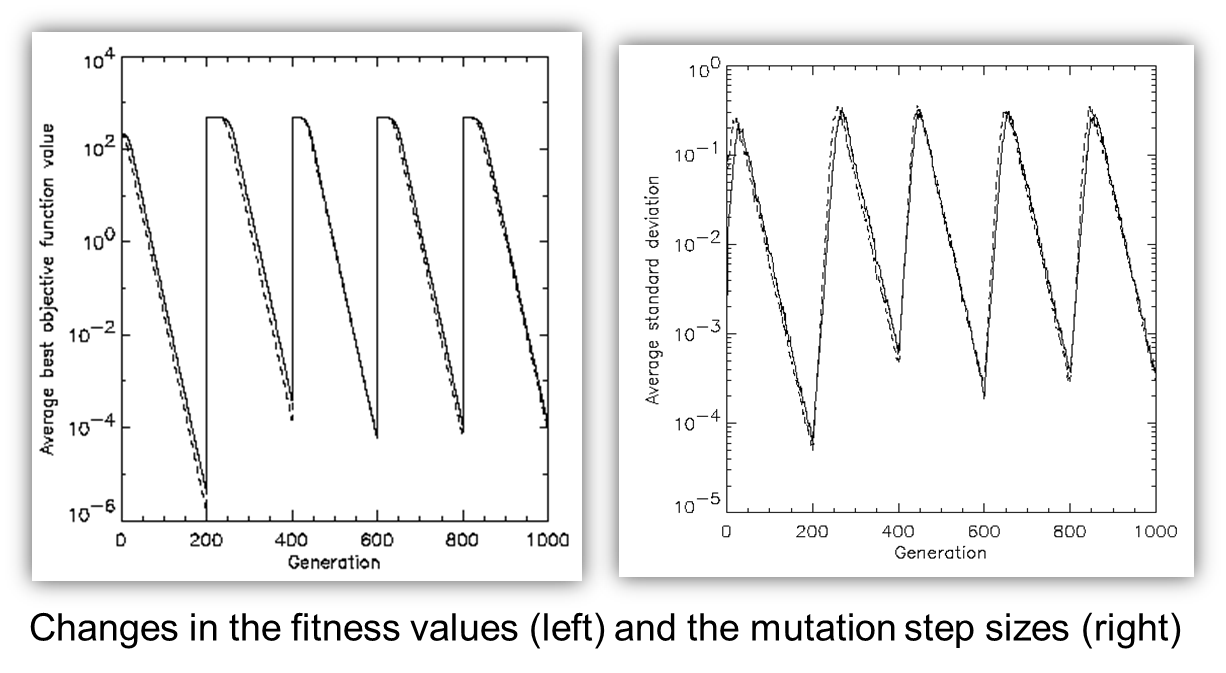
Since the 1990s,
EP variants for optimization of real-valued parameter vectors have
become more frequent,
and even positioned as “standard’ EP.
During the history of EP a number of mutation schemes,
such as one in which the step size is inversely related to the fitness
of the solutions,
have been proposed.
Since the proposal of meta-EP,
self-adaptation of step sizes has become the norm.
Other ideas from ES have also informed the development of EP
algorithms,
and a version with self-adaptation of covariance matrices, called
R-meta-EP is also in use.
Worthy of note is Yao’s improved fast evolutionary programming algorithm
(IFEP).
whereby two offspring are created from each parent,
one using a Gaussian distribution to generate the random
mutations,
and the other using the Cauchy distribution.
The latter has a fatter tail
(i.e., more chance of generating a large mutation),
which the authors suggest gives the overall algorithm greater chance of
escaping from local minima,
whilst the Gaussian distribution (if small step sizes evolve),
gives greater ability to fine-tune the current parents.
Little to none, though it was present:
http://scholarpedia.org/article/Evolutionary_programming
Rationale:
One point in the search space stands for a species,
not for an individual and there can be no crossover between
species.
Much historical debate “mutation vs. crossover”.
The issue of using a mutation-only algorithm versus a recombination and
mutation variant has been intensively discussed since the 1990s.
“the traditional practice of setting operator probabilities at constant
,
… is quite limiting and may even prevent the successful discovery of
suitable solutions.”
06-PopularVariants/fogel02.pdf
Skim paper, figure of ANN at end.
Tournament size q = 5
Programs (with NN inside) play against other programs,
no human trainer or hard-wired intelligence.
After 840 generation (6 months!),
best strategy was tested against humans via Internet.
Program earned “expert class” ranking,
outperforming 99.61% of all rated players.
NeuroEvolution
The checkers player is a kind of:
https://en.wikipedia.org/wiki/Neuroevolution
http://www.scholarpedia.org/article/Neuroevolution
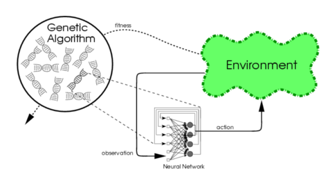
Evolutionary algorithms generate artificial neural networks (ANN),
their parameters, and their rules.
It is commonly used as part of the reinforcement learning
paradigm,
and it can be contrasted with conventional deep learning
techniques,
that use gradient descent on a neural network with a fixed topology.
Discussion question:
What happened to the field of EP’s evolving FSMs?
https://en.wikipedia.org/wiki/Genetic_programming
https://geneticprogramming.com/
https://www.genetic-programming.com/
The first record of the proposal to evolve programs is probably that
of Alan Turing in the 1950s.
06-PopularVariants/turing50.pdf
Non-GP EC grew in the 60s and 70s,
but despite this progress,
there was a gap of some thirty years,
before Richard Forsyth demonstrated the successful evolution of small
programs,
represented as trees,
to perform classification of crime scene evidence for the UK Home
Office!
06-PopularVariants/beagle81.pdf
Although the idea of evolving programs,
initially in the computer language LISP,
was discussed among John Holland’s students,
it was not until they organized the first Genetic Algorithms conference
in Pittsburgh,
that Nichael Cramer published evolved programs in two specially designed
languages.
https://dl.acm.org/doi/10.5555/645511.657085
In 1988, another PhD student of John Holland,
John Koza, patented his invention of a GA for program evolution:
“Non-Linear Genetic Algorithms for Solving Problems”,
“United States Patent 4935877”, 1990
This was followed by publication in the International Joint
Conference on Artificial Intelligence IJCAI-89.
06-PopularVariants/koza_ijcai1989.pdf
Then, Koza followed this with 205 publications on “Genetic
Programming” (GP).
GP was a name coined by David Goldberg, also a PhD student of John
Holland.
There was an enormous expansion of the number of publications.
In 2010, Koza listed 77 results where Genetic Programming was human
competitive.
06-PopularVariants/koza_GPEM2010article.pdf
Genetic programming is a relatively young member of the evolutionary
algorithm family.
EAs discussed so far are typically applied to optimization
problems.
Most other EAs find some input, realizing maximum payoff.
GP could instead be positioned in machine learning.
GP is used to seek models with maximum fit.
Once maximization is introduced,
modeling problems can be seen as special cases of optimization.
This is the basis of using evolution for such tasks:
models, represented as parse trees,
are treated as individuals,
and their fitness is the model quality to be maximized.
Discussion question:
Might GP subsume other fields?
Does GP suffice in all cases where evolving an FSM might?
Would you guess GP has any disadvantages compared to simpler
representations?
The parse trees used by GP as chromosomes are expressions in a given
formal syntax.
Depending on the problem at hand,
and the users’ perceptions on what the solutions must look like,
this can be the syntax of arithmetic expressions,
formulas in first-order predicate logic,
or code written in a programming language.
In particular, they can be envisioned as executable source code,
that is, programs.
The syntax of functional programming,
e.g., the language LISP,
very closely matches the so-called Polish notation of expressions.
For instance, the formula we covered before:
\(2 \cdot \pi + ((x + 3) -
\frac{y}{5+1})\)
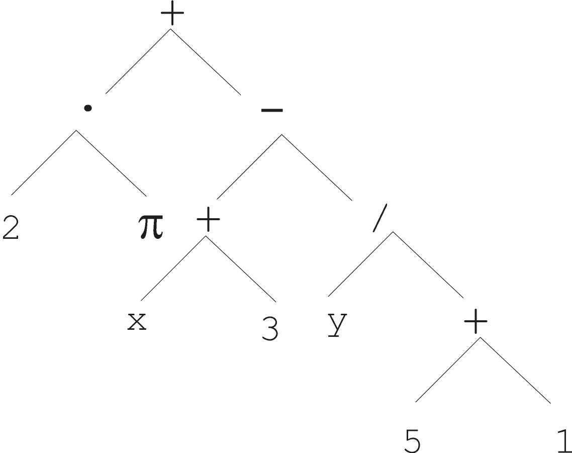
can be rewritten in this Polish notation as:
+(·(2, π), −(+(x, 3), /(y, +(5, 1)))),
while the executable LISP code1 looks like:
(+ (· 2 π) (− (+ x 3) (/ y (+ 5 1)))).
This is cool!
| Meta-part | Option |
|---|---|
| Representation | Tree structures |
| Recombination | Exchange of subtrees |
| Mutation | Random change in trees |
| Parent selection | Fitness proportional |
| Survivor selection | Generational replacement |
Most are basic trees:
But, there are other flavors too (more below).
Bank wants to distinguish good from bad loan applicants
Model needed that matches historical data
| ID | No of children (NoS) | Salary (S) | Marital status | OK? |
|---|---|---|---|---|
| ID-1 | 2 | 45000 | Married | 0 |
| ID-3 | 1 | 40000 | Divorced | 1 |
| ID-2 | 0 | 30000 | Single | 1 |
| … |
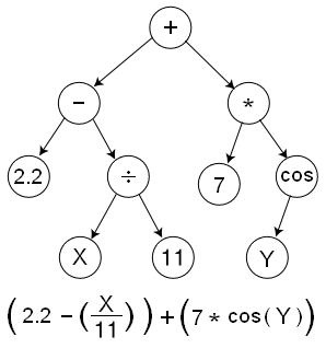
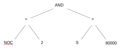
A possible model:
IF (NoC = 2) AND (S > 80000)
THEN good
ELSE bad
In general:
IF formula
THEN good
ELSE bad
Only unknown is the right formula, hence:
Our search space (phenotypes) is the set of formulas.
Natural fitness of a formula:
percentage of well classified cases of the model it stands for.
IF (NoC = 2) AND (S > 80000)
THEN good
ELSE bad
can be represented by the following tree
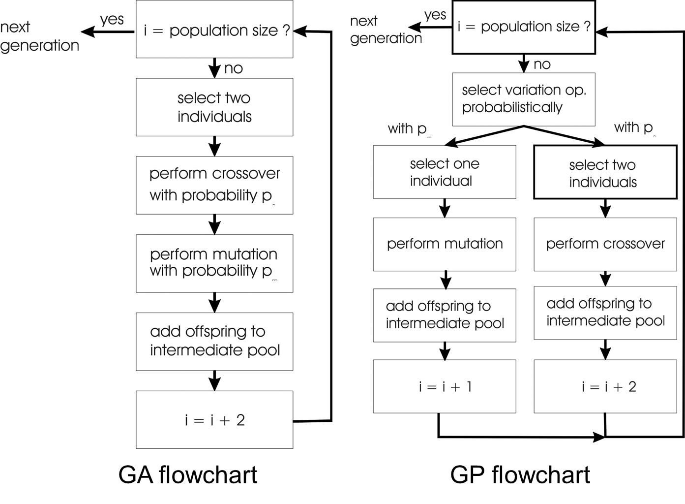
Compare:
GA scheme using crossover AND mutation sequentially (be it
probabilistically)
GP scheme using crossover OR mutation (chosen probabilistically)
Average tree sizes tend to grow during the course of a run.
This is known as bloat,
sometimes called the ‘survival of the fattest’.
This may be a broader phenomenon than GP.
Bloat is seemingly observed in organismal chromosomes as well.
Some small viruses show size constraints.
The simplest way to prevent bloat,
is to introduce a maximum tree size.
If the child(ren) resulting from a variation aperation would exceed this
maximum size,
then the variation operator is forbidden from acting.
The threshold can be seen as an additional parameter of mutation and
recombination in GP.
Another mechanism is parsimony pressure.
(i.e., being ‘stingy’ or ungenerous)
is achieved through introducing a penalty term in the fitness
formula,
that reduces the fitness of large chromosomes,
or uses other multiobjective techniques.
Types of GP include:
Tree-based Genetic Programming
Stack-based Genetic Programming
Linear Genetic Programming (LGP)
Grammatical Evolution
Extended Compact Genetic Programming (ECGP)
Cartesian Genetic Programming (CGP)
Probabilistic Incremental Program Evolution (PIPE)
Strongly Typed Genetic Programming (STGP)
Genetic Improvement of Software for Multiple Objectives (GISMO)
Review this briefly:
https://geneticprogramming.com/software/
Mention Clojush, Tiny Genetic Programming
http://www.gp-field-guide.org.uk/
06-PopularVariants/GP_book1.pdf
https://www.moshesipper.com/books/evolved-to-win/
06-PopularVariants/evolvedtowin.pdf
Mention his GP bot competitions.
And, our future lecture for this course:
18-GeneticProgramming.html
https://en.wikipedia.org/wiki/Learning_classifier_system
Is much like an independent discovery of processes which
resemble:
reinforcement learning, Q-learning, TD-learning.
https://en.wikipedia.org/wiki/Reinforcement_learning
https://en.wikipedia.org/wiki/Temporal_difference_learning
https://en.wikipedia.org/wiki/Q-learning (show
images)
Read (show this briefly):
https://artint.info/2e/html/ArtInt2e.Ch12.html
https://artint.info/3e/html/ArtInt3e.Ch13.html
Animation on ch12 here (Java applets, lol):
https://artint.info/2e/online.html
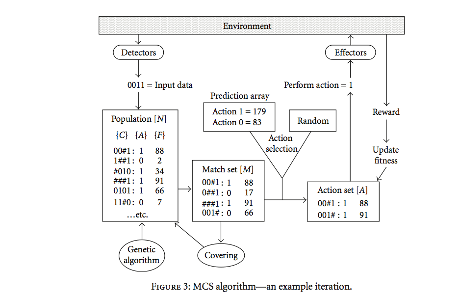
Genome:
{condition:action:payoff}
{condition:action:payoff,accuracy}
Where payoff is like RL’s reward.
| Meta-part | Option |
|---|---|
| Representation | Tuple of {condition:action:payoff,accuracy}, conditions use {0,1,#} alphabet |
| Survivor selection | Stochastic, inversely related to number of rules covering same environmental niche |
| Recombination | One-point crossover on conditions/actions |
| Parent selection | Fitness proportional with sharing within environmental niches |
| Mutation | Binary resetting as appropriate on action/conditions |
| Fitness | Each reward received updates predicted pay-off and accuracy of rules in relevant action sets by reinforcement learning |
Each rule of the rule base is a tuple {condition:action:payoff}
Match set: subset of rules whose condition matches the current inputs
from the environment
Action set: subset of the match set advocating the chosen action
Later, the rule-tuple included an accuracy value,
reflecting the system’s experience of how well the predicted payoff
matches the reward received
The Pittsburgh-style LCS predates,
but is similar to the better-known GP:
Each member of the evolutionary algorithm’s population represents a
complete model,
of the mapping from input to output spaces.
Each gene in an individual typically represents a rule,
and a new input item may match more than one rule,
in which case typically the first match is taken.
This means that the representation should be viewed as an ordered
list.
Two individuals which contain the same rules,
but in a different order on the genome,
are effectively different models.
Learning of appropriately complex models is typically facilitated by
using a variable-length representation,
so that new rules can be added at any stage.
This approach has several conceptual advantages.
In particular, since fitness is awarded to complete rule sets,
models can be learned for complex multi-step problems.
The downside of this flexibility is that,
like GP, Pittsburgh-style LCS suffers from bloat,
and the search space becomes potentially infinite.
Nevertheless, given sufficient computational resources,
and effective methods of parsimony to counteract bloat,
Pittsburgh-style LCS has demonstrated state-of-the-art performance in
several machine learning domains,
especially for applications such as bioinformatics and medicine,
where human-interpretability of the evolved models is vital,
and large data-sets are available,
so that the system can evolve off-line to minimize prediction
error.
Two recent examples winning Humies Awards,
for better than human performance are in the realms of:
prostate cancer detection and protein structure prediction.
https://en.wikipedia.org/wiki/Differential_evolution
| Meta-part | Option |
|---|---|
| Representation | Real-valued vectors |
| Recombination | Uniform crossover |
| Mutation | Differential mutation |
| Parent selection | Uniform random selection of the 3 necessary vectors |
| Survivor selection | Deterministic elitist replacement (parent vs child) |
In this section we describe a young member of the evolutionary
algorithm family:
differential evolution (DE).
Its birth can be dated to 1995,
when Storn and Price published a technical report describing the main
concepts behind a
“new heuristic approach for minimizing possibly nonlinear and
non-differentiable continuous space functions”.
The distinguishing feature that delivered the name of this
approach,
is a twist to the usual reproduction operators in EC:
the so-called differential mutation.
Given a population of candidate solution vectors in the set of real
numbers, \({\rm I\!R}^n\),
a new mutant vector x’ is produced,
by adding a perturbation vector to an existing one,
x’ = x + p,
where the perturbation vector, p, is the scaled vector difference
of:
two other, randomly chosen population members
p = F · (y − z),
where y and x are randomly chosen population members,
the scaling factor F > 0 is a real number,
that controls the rate at which the population evolves.
DE uses uniform crossover but with a slight twist
The other reproduction operator is the usual uniform crossover,
subject to one parameter,
the crossover probability Cr ∈ [0, 1]
that defines the chance that for any position in the parents currently
undergoing crossover,
the allele of the first parent will be included in the child.
Remember that in GAs, the crossover rate pc ∈ [0, 1] is defined for
any given pair of individuals,
and it is the likelihood of actually executing crossover.
In DE, at one randomly chosen position,
the child allele is taken from the first parent, without making a random
decision.
This ensures that the child does not duplicate the second parent.
The number of inherited mutant alleles follows a binomial
distribution
https://en.wikipedia.org/wiki/Particle_swarm_optimization
http://scholarpedia.org/article/Particle_swarm_optimization
| Meta-part | Option |
|---|---|
| Representation | Real-valued vectors |
| Recombination | None |
| Mutation | Adding velocity vector |
| Parent selection | Deterministic (each parent creates one offspring via mutation) |
| Survivor selection | Generational (offspring replaces parents) |
Every population member can be considered as a pair,
where the first vector is candidate solution,
and the second one a perturbation vector in \({\rm I\!R}^n\)
On a conceptual level every population member in a PSO can be
considered as a pair <x, p>,
where \({x \in \rm I\!R}^n\) is a
candidate solution vector and \({p \in \rm
I\!R}^n\) is a perturbation vector,
that determines how the solution vector is changed to produce a new
one.
The main idea is that a new pair <x’, p’> is produced from <x,
p>
by first calculating a new perturbation vector p’
(using p and some additional information)
and adding this to x.
That is,
x’ = x + p’
The core of the PSO perspective is to consider a population member as a
point in space,
with a position and a velocity,
and use the latter to determine a new position (and a new
velocity).
Thus, looking under the hood of a PSO,
we find that a perturbation vector is a velocity vector v,
and a new velocity vector v’ is defined as:
the weighted sum of three components: v and two vector
differences.
The first points from the current position x to the best position y the
given population member ever had in the past,
and the second points from x to the best position z the whole population
ever had.
The perturbation vector determines how the solution vector is changed to produce a new one.
https://en.wikipedia.org/wiki/Estimation_of_distribution_algorithm
Estimation of distribution algorithms (EDA) are based on the idea of
replacing the creation of offspring by ‘standard’ variation operators
(recombination and mutation) by a three-step process.
First a ‘graphical model’ is chosen to represent the current state of
the search,
in terms of the dependencies between variables (genes) describing a
candidate solution.
Next the parameters of this model are estimated from the current
population,
to create a conditional probability distribution over the
variables.
Finally, offspring are created by sampling this distribution.
BEGIN
    INITIALISE population P 0 with µ random candidate solutions;
    set t = 0;
        REPEAT UNTIL ( TERMINATION CONDITION is satisfied ) DO
        EVALUATE each candidate in P t ;
        SELECT subpopulation Pst to be used in the modeling steps;
        MODEL SELECTION creates graph G by dependencies in Pst ;
        MODEL FITTING creates Bayesian Network BN with G and Pst ;
        MODEL SAMPLING produces a set Sample(BN ) of µ candidates;
        set t = t + 1;
        P t = Sample(BN );
    OD
ENDhttps://en.wikipedia.org/wiki/Evolutionary_robotics
http://scholarpedia.org/article/Evolutionary_Robotics
https://en.wikipedia.org/wiki/Neuroevolution
http://www.scholarpedia.org/article/Neuroevolution
Discussed above!